GridVisio Documentation
GridVisio is a professional coverage mapping and network planning tool built for Wireless Internet Service Providers (WISPs). It helps operators visualize their network, identify coverage gaps, manage subscribers, and collaborate with their team — all from a browser.
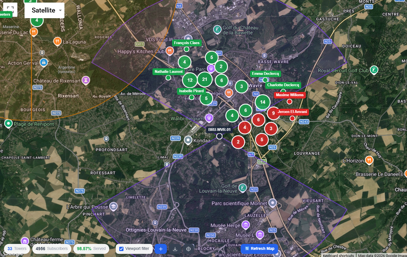
What GridVisio does
Network visualization
Plot towers with directional or omnidirectional sector coverage on an interactive satellite map.
Subscriber management
Import, map, and track thousands of subscribers with automatic coverage status calculation.
Coverage analysis
Detect unserved areas (white areas) and identify overlapping coverage between sectors.
Export & reporting
Export coverage data as PDF, PNG, XLSX, or in BDC/BEAD formats for government filings.
Sharing
Share read-only map views with clients, stakeholders, or regulators via a secure link.
Team collaboration
Invite editors and viewers to projects with role-based access control.
Who It's For
GridVisio is designed for:
- WISP operators — small to mid-size wireless internet providers managing fixed wireless infrastructure
- Network engineers — planning new tower deployments and sector coverage
- Operations managers — tracking subscriber coverage status and identifying growth areas
- Grant applicants — preparing BDC (Broadband Data Collection) and BEAD program filings
- Field technicians — looking up tower coordinates in Lambert or WGS84 format
GridVisio works for WISPs of any size and in any country. All geographic coordinate systems are supported. Regional tools (such as the Lambert coordinate converter for Belgian operators) are available alongside standard lat/lng workflows without limiting users in other regions.
Technical Overview
GridVisio is a web application accessible from any modern browser. No installation is required.
Browser
Chrome, Firefox, Edge, Safari. Best experience on desktop. Tablet-compatible.
Maps
Google Maps JavaScript API with satellite, hybrid, and roadmap views.
Security
All data is private to your account. Shared maps use token-based access with optional expiry.
Account & Plans
Every GridVisio account starts with a 14-day free trial giving full Starter-level access with no credit card required. After the trial you choose a plan to continue.
Plan badge
Your current plan is always visible in the bottom-left corner of the sidebar as a coloured badge on your user widget: amber for Trial, gray for Free, blue for Starter, purple for Pro.
Projects
A project is the top-level container for a network deployment. Each project has its own towers, subscribers, shared maps, and team members.
Sidebar → Network → ProjectsCreating a project
- 1Click "New Project"
From the Projects list, click the New Project button in the top right.
- 2Fill in project details
Name (required), description, country, and region. These appear on the project dashboard.
- 3Save and configure
After saving you'll be taken to the project view where you can add towers, configure settings, and invite team members.
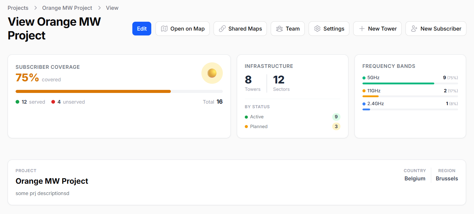
Project dashboard
The project view page shows live statistics for the project:
- Subscriber coverage % — percentage of served subscribers with a progress bar
- Subscriber breakdown — served / unserved / potential / unknown counts
- Infrastructure — tower and sector counts, sectors by status (active/planned/offline)
- Frequency bands — breakdown of sectors by frequency with usage bars
Project actions
From the project view header:
- Open on Map — opens the coverage map centred on this project
- New Tower — create a tower pre-assigned to this project
- New Subscriber — create a subscriber pre-assigned to this project
- Shared Maps — manage shareable read-only links
- Team — invite and manage collaborators
- Settings — configure project-specific defaults
Towers & Sectors
A tower represents a physical site where antennas are mounted. Each tower has one or more sectors, each defining a beam of coverage (direction, width, radius, frequency).
Sidebar → Network → Towers Coverage Map → + → Add Tower → click map Coverage Map → click existing tower marker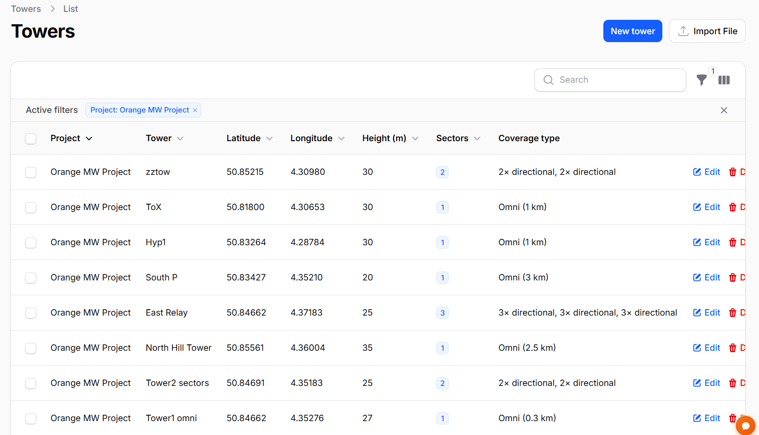
Tower fields
- Name — display name shown on the map
- Latitude / Longitude — position; click on the map picker to set
- Tower / structure height (shown in m or ft per your Distance Unit preference) — the physical structure's height (the mast, rooftop, water tower, etc. the antennas are mounted on) — not an antenna height itself. It's the reference ceiling each sector's antenna height below can't exceed, and the starting default for a new sector's antenna height.
- Notes — free-text site notes
Sector fields
- Name — e.g. "North 5GHz", "Omni"
- Azimuth (°) — direction the sector points (0=North, 90=East, 180=South, 270=West)
- Beamwidth (°) — horizontal angular width of the beam. Use 360 for omnidirectional
- Radius (shown in km or mi per your Distance Unit preference) — coverage distance. Determines the size of the coverage shape on the map. Must be greater than 0 and at most 35 km on every plan — for a genuine point-to-point backhaul link longer than that, use the LoS Link Check tool instead of a Sector. See Classification below for how a subscriber just outside this radius can still qualify as Served.
- Antenna height (m or ft, same preference) — this specific sector's antenna mounting height on the tower. Different sectors on the same physical tower are often mounted at different heights (e.g. a 5GHz sector near the top, a 900MHz sector lower down) — this field lets the LoS checker use the real height for whichever sector actually serves a given direction, instead of one flat tower-wide number. Must be greater than 0 and cannot exceed the parent tower's structure height; defaults to the tower's current height when a new sector is added, but can be lowered.
- Frequency band — selected from this project's own frequency list (configured in Project Settings, starts from a default set of 19 common bands and is fully editable). A small "?" hint next to the field explains where to add a precise value if what you need isn't in the list. See also Equipment Presets — the adjacent "Preset" selector fills this and five other RF fields in one click.
- Colour — fill colour of the coverage shape on the map
- Status — active / planned / offline. See the callout below for what this controls beyond the map legend colour.
- TX power (dBm) — this sector's radio's conducted output power. Typical WISP AP gear runs 20–27 dBm. Used only by the RF Propagation Heatmap feature, not by the LoS Link Check or Coverage Widget.
- Antenna gain (dBi) — this sector's antenna boresight gain. Typical WISP sector antennas run 16–22 dBi (up to ~41 dBi for 60 GHz mmWave gear, e.g. Ubiquiti Wave Nano). Same scope as TX power above — heatmap only.
- Downtilt (°) — mechanical or electrical antenna tilt relative to horizontal. Negative = downtilt (e.g. −5 = 5° below horizontal), 0 = horizontal boresight. Typical WISP AP values: −3° to −8°. Used only by the heatmap — the vertical pattern adjustment reduces effective gain for grid points well above or below the boresight angle. Default: 0.
- Vertical beamwidth (°) — the 3 dB (half-power) beamwidth of the antenna in the vertical plane. Check your antenna datasheet; typical values: 7° for high-gain narrow-beam sectors, 10–14° for wider beams. Together with downtilt, this determines how quickly gain rolls off away from boresight. Default: 10°. Used only by the heatmap.
A sector's Status (active / planned / offline) controls more than its colour in the legend — different tools across GridVisio deliberately follow one of three policies:
- All statuses count (status-agnostic) — the baseline geometric served/unserved test (see Subscribers), the RF Propagation Heatmap, and the LoS Link Check tool. These either establish the underlying truth or are explicit planning/inspection features, not a live-service claim — a Planned (not-yet-built) or Offline (decommissioned) sector's geometry, and for LoS Link Check its real configured TX power/gain/frequency too, are used exactly as an Active sector's would be. The sector's own status is always shown alongside the result, never hidden, so it's never mistaken for a live measurement.
- Active only — anything answering "can this exact point actually be served right now": the Classification RSSI/throughput verification's search for a candidate tower, the public Coverage Widget, POP Scan, and Rooftop Scan. A Planned or Offline sector never shows up as a live candidate in any of these — a Coverage Widget visitor, for instance, is never told they're covered by a sector that isn't built yet.
- Active + Planned (Offline excluded) — Interference Analysis: it exists to catch a frequency conflict before a Planned sector goes live, but ignores Offline/decommissioned gear as irrelevant noise.
Classification is actually a hybrid of the first two: the base served/unserved status is status-agnostic (the geometric test doesn't care whether the matching sector is Active, Planned, or Offline), but the RSSI/throughput verification pass only searches Active sectors for a potentially better-performing candidate — a subscriber's own already-resolved serving sector is always still measured even when it isn't Active, it just can't be outranked by a Planned/Offline alternative elsewhere.
A couple of narrower, tool-specific defaults follow the "Active only" rule too: the BEAD/white-area bulk check and the LoS Link Check tool's antenna-height pre-fill both fall back to the tower's own structure height when the only sector pointing that direction is Planned or Offline (as if the tower had no sector there at all); the per-tower frequency used in the Coverage Widget's and BEAD check's path-loss calculation is likewise taken only from an Active sector, defaulting to 5.8 GHz if the tower has none.
Adding a tower from the map
Click + → Add Tower, then click the map. The tower form opens immediately with a pre-configured default Omni sector already shown. You can adjust the name, height, sector radius, antenna height, colour, and frequency before saving — or just click Add Tower to accept the defaults and place the tower instantly. Default sector values (radius, frequency, colour, beamwidth) are taken from Project Settings; antenna height defaults to the tower's own height.
Editing an existing tower
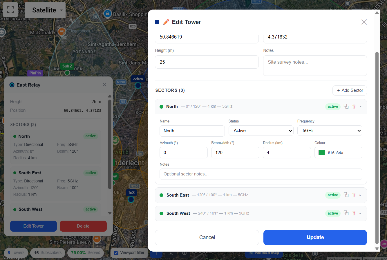
Click any tower marker on the map to open the edit modal directly. The modal shows all tower fields plus a collapsible sector repeater where you can add, edit, clone, and delete sectors. Click Update to save.
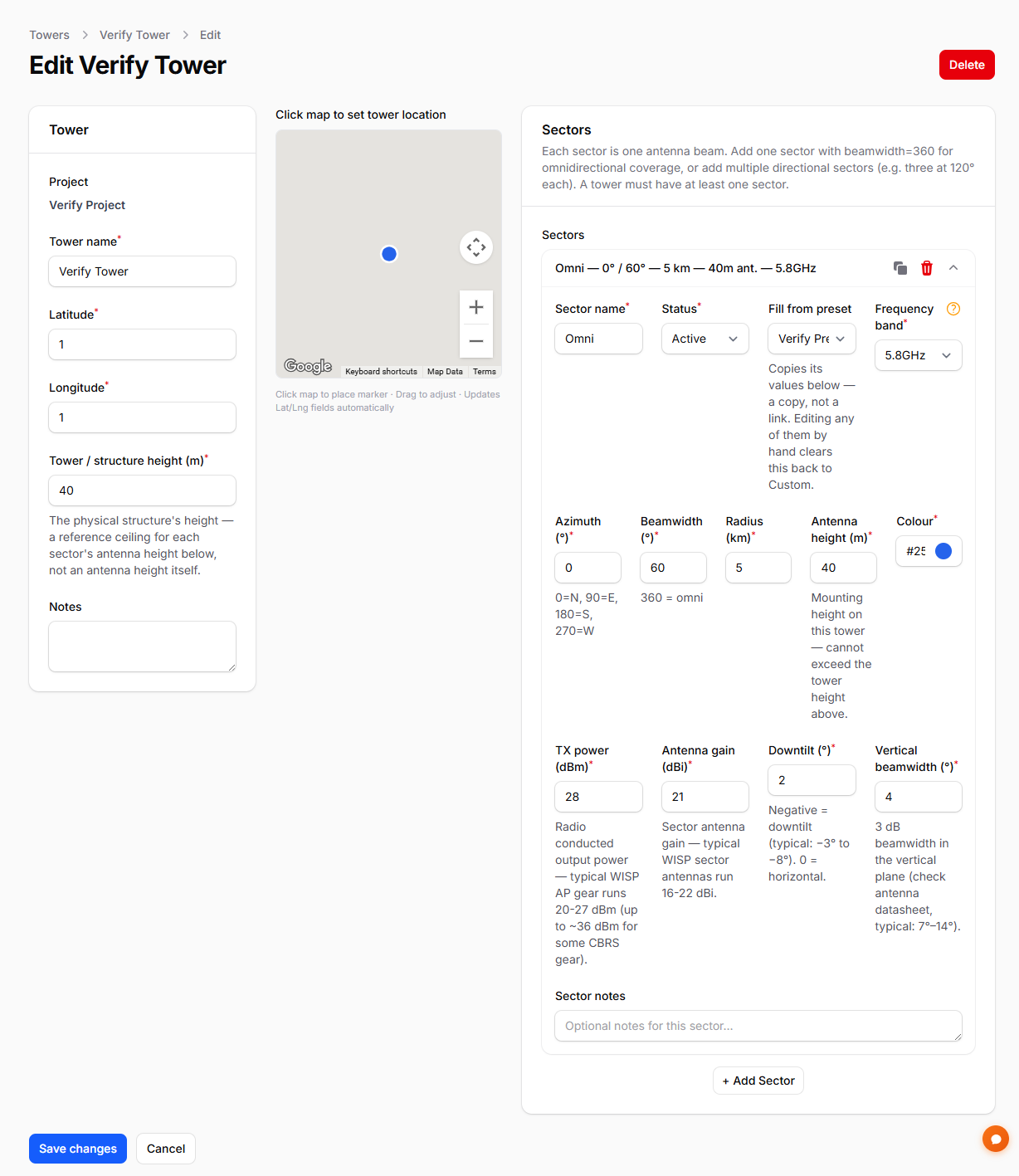
Each sector's Preset dropdown (next to Name, Status, and Colour) fills the six RF fields — frequency, beamwidth, TX power, antenna gain, downtilt, and vertical beamwidth — from a saved equipment preset in one click. See the screenshot below: selecting a preset copies its values as a one-time fill, not a live link, so hand-editing any of those fields afterward automatically resets the dropdown to — Custom —.
Importing towers
See the Importing Data section for CSV/XLSX import format and field mapping.
Equipment Presets
An equipment preset is a named, reusable bundle of the six RF fields a sector needs — frequency band, beamwidth, TX power, antenna gain, downtilt, and vertical beamwidth. Save the specs for a radio/antenna combination you actually run once, then fill a sector from it in one click instead of re-typing the same numbers on every tower. Presets are manufacturer-agnostic — GridVisio doesn't care whether the underlying hardware is Ubiquiti, Cambium, Mimosa, or anything else; a preset is just a set of numbers you define.
Sidebar → Network → Equipment PresetsPresets are account-level, enabled per project
Presets belong to your account, not to any one project — save one and it's available everywhere you work. Whether it's actually offered when editing a sector is controlled per project, in that project's Settings → Equipment Presets tab. A new project starts with every existing preset enabled; disabling one there just stops it appearing in that project's Preset dropdown; it doesn't touch the preset itself or any sector already filled from it.
Creating a preset
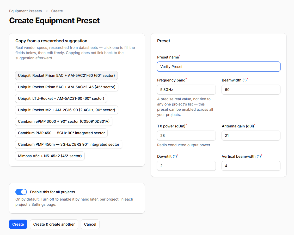
Click New equipment preset. Above the fields, a row of buttons offers real vendor specs researched from datasheets — Ubiquiti, Cambium, and Mimosa sector radios — as starting points: click one to fill in the frequency, beamwidth, TX power, antenna gain, downtilt, and vertical beamwidth fields, then edit freely before saving. Copying from a suggestion is a one-time fill, not a link back to it — the saved preset is fully independent afterward. You can also skip the suggestions and enter your own values directly for hardware not on the list.
The Enable this for all projects checkbox (on by default) enables the new preset across every one of your existing projects immediately; turn it off to enable it by hand later, per project, in each project's Settings page.
Enabling a preset for a project automatically adds that preset's frequency to the project's own frequency list if it isn't already there — so the preset is always immediately usable. Because of this, a frequency still in use by an enabled preset can't be removed from a project's frequency list until that preset is disabled for the project first.
Filling a sector from a preset
Wherever a sector is edited — the map's tower edit modal and the admin tower-edit form both — a Preset selector sits next to the sector's Name, Status, and Colour fields. Its options are labelled "name — frequency" so you can see at a glance which band each preset uses; an option is greyed out with an explanatory tooltip if its frequency isn't on the current project's frequency list. Selecting a preset copies its six RF values into the sector's fields as a one-time fill.
The dropdown always reflects the sector's current values, recomputed after every change — it isn't edit history. Opening a sector that already happens to match a preset's values shows that preset pre-selected; hand-editing any of the six copied fields afterward clears the selector back to — Custom —; reproducing another preset's exact values re-selects that preset automatically.
Subscribers
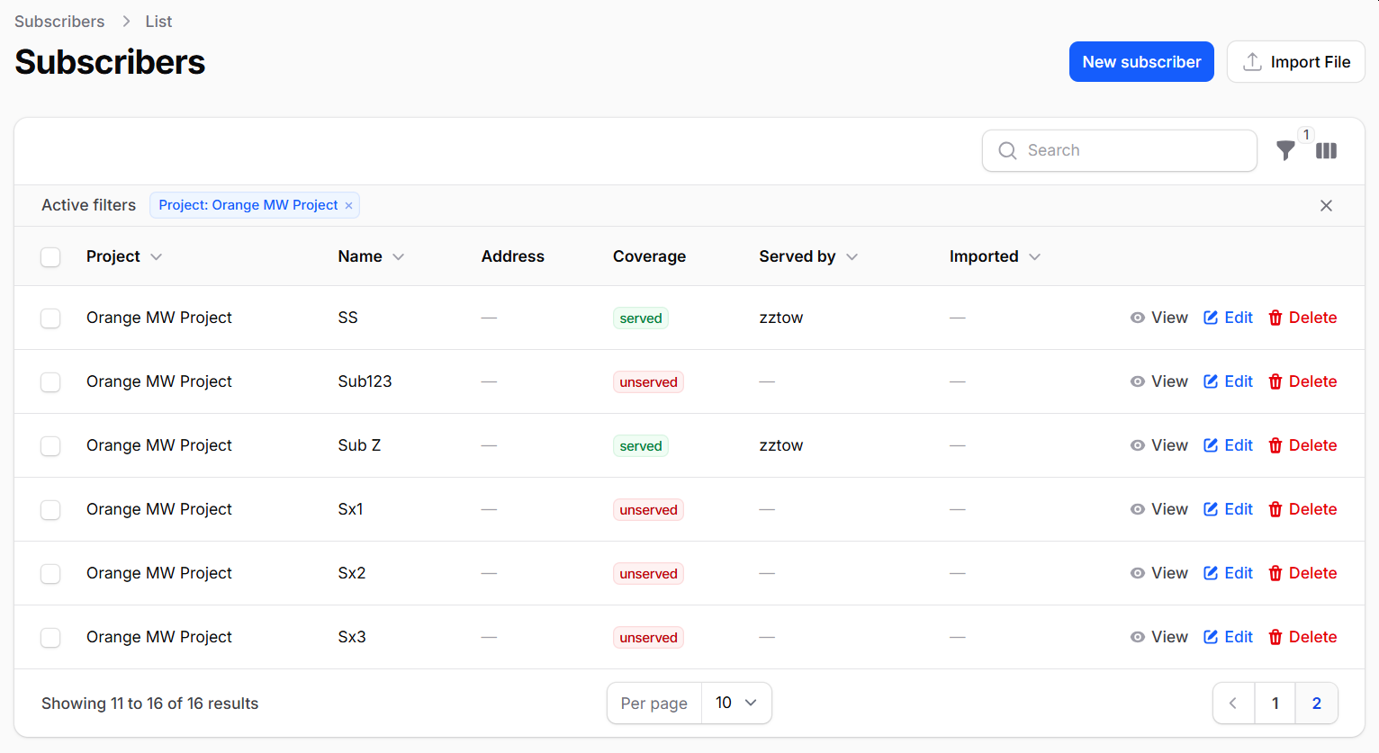
A subscriber is a customer or installation point. Subscribers are plotted on the map and their coverage status is automatically calculated based on whether they fall within any sector's coverage area.
Sidebar → Network → SubscribersCoverage status
- Served — subscriber falls within at least one active sector's coverage area (and, if RSSI verification is on, predicted signal is at or above the threshold)
- Marginal — geometrically served, but RSSI verification is on and predicted signal has fallen below the threshold while still above the hard floor. See Classification below.
- Unserved — subscriber has coordinates but is outside all coverage areas, or predicted signal has fallen below the hard floor
- Unknown — no coordinates yet, or coverage not yet calculated
"Potential" (a manually-flagged prospect, independent of coverage) still exists as a separate marker layer/filter elsewhere in the app but is not one of the four coverage-status values above.
Coverage is calculated server-side using a geometric point-in-sector test. For each subscriber with coordinates, the system checks every sector in the project regardless of status — active, planned, and offline sectors are all considered equally — and stops at the first sector that matches. A subscriber is "served" if the distance from the tower is within the sector's radius AND the bearing to the subscriber falls within the sector's azimuth ± beamwidth/2. The calculation runs automatically when towers or sectors are created, edited, or deleted. If RSSI/throughput verification is turned on for the project, every active sector that reaches the subscriber (not just the one the geometric test happened to pick) is then re-tested with a real signal prediction from this project's configured propagation model(s) — the same engine the RF Heatmap and LoS Link Check tools use — and the single best-performing candidate can downgrade a geometrically-served subscriber to Marginal or Unserved, promote a nearby beyond-radius subscriber to Served (if the extend-beyond-radius option is also on), or even hand "serving tower" duty to a different tower/sector than the geometric test chose. See the callouts under Classification below for the full detail on multi-candidate matching, the active-only requirement, and CPE frequency compatibility.
Subscriber fields
- Name — customer name or site identifier
- Address — physical address (for reference, not geocoded automatically)
- Latitude / Longitude — position; click on the map picker to set
- Height (m or ft per your Distance Unit preference) — subscriber module (SM) / antenna mounting height above ground. Default 5 m; must be greater than 0 and at most 1000 m. Pre-fills automatically in the LoS Link Check tool when this subscriber is selected as an endpoint.
- Status — calculated automatically (served/marginal/unserved) or set manually (potential)
Predicted signal popover
Hovering a subscriber marker on the map (when RSSI verification is on for the project, and your plan includes it) shows a small popover with the predicted signal for that subscriber: predicted RSSI against the configured threshold, predicted throughput against the configured minimum (if throughput qualification is also on), and which tower/sector the prediction is measured against. For a subscriber promoted beyond its sector's configured radius, or measured against non-serving infrastructure while still Unserved, this is the only place that measured tower/sector identity is shown — the subscriber's own Tower/Sector fields only change on a real promotion.
Importing Data
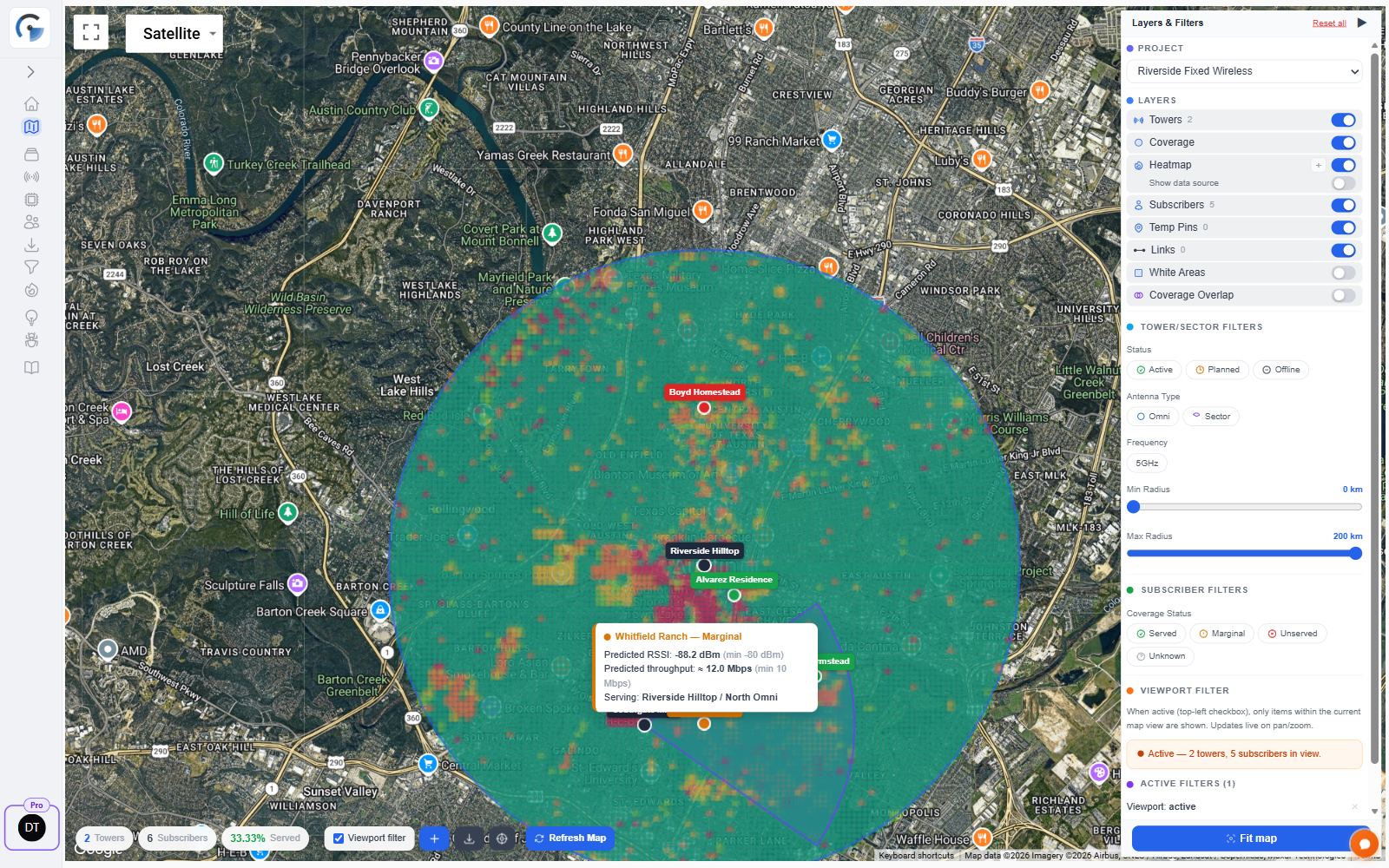
GridVisio supports bulk import of subscribers via CSV/XLSX, and towers & sectors via CSV/XLSX or three additional sources — Shapefile, KML/KMZ, or directly from a cnHeat account's API. Import is available from the Towers and Subscribers list pages.
Towers list → Import Towers Subscribers list → ImportImport requires a Starter or Pro plan — this applies the same way to every tower source (CSV/XLSX, Shapefile, KML/KMZ, cnHeat API) and to subscriber CSV/XLSX. Drive test import also requires Starter or Pro.
Choosing a source
The Towers list's Import Towers button opens one dialog with a 4-way Import from selector (CSV/Excel, Shapefile, KML/KMZ, cnHeat API) at the top — the fields below it change to match whichever is selected. Every source feeds the same underlying process: find-or-create the tower by location, create one sector per source row/feature, validate every RF field with the same rules, and finish with the same import log, activity record, and automatic coverage recalculation. The Subscribers list's own Import stays CSV/XLSX only.
Tower import format
Accepted columns (CSV headers, case-insensitive) — the sample file offered in the import dialog uses radius_km/height_m/antenna_height_m or radius_mi/height_ft/antenna_height_ft to match your own Distance Unit preference:
tower_name, lat, lng, height_m (or height_ft), notes, sector_name, azimuth, beamwidth, radius_km (or radius_mi), antenna_height_m (or antenna_height_ft), tx_power_dbm, antenna_gain_dbi, tilt_deg, vertical_beamwidth_deg, frequency_band, color, status
- tower_name, lat, lng — required
- radius_km (or radius_mi) — required per sector row; a file may use either column name regardless of your account's own Distance Unit setting — GridVisio converts and stores it correctly either way. Must be greater than 0 and at most 35 km (21.7 mi) — a row outside that range is skipped with a warning in the import log, stated in whichever unit that row's own column used.
- height_m (or height_ft) — optional, tower/structure height; defaults to 30 m (98.43 ft) if empty. Either column name is accepted regardless of your account's own Distance Unit setting.
- beamwidth, frequency_band, color — fall back to project defaults if empty
- antenna_height_m (or antenna_height_ft) — optional; defaults to that row's tower height if empty. Must be greater than 0 and not exceed the tower's height — a row with an out-of-range value is skipped with a warning in the import log, stated in whichever unit that row's own column used, same treatment as an invalid lat/lng.
- tx_power_dbm — optional; defaults to 24. Must be between 0 and 37 — out-of-range skips the row.
- antenna_gain_dbi — optional; defaults to 17. Must be between 0 and 50 — out-of-range skips the row.
- tilt_deg — optional; defaults to 0 (horizontal boresight). Negative = downtilt (e.g. −5). Must be between −90 and 90 — out-of-range skips the row.
- vertical_beamwidth_deg — optional; defaults to 10. Must be between 1 and 90 — out-of-range skips the row.
- Multiple sectors per tower: repeat the tower row with the same name and different sector columns
Frequency values are normalized on import for spelling/format only — common variants (e.g. "5.8", "5800MHz", "5.8GHz") all map to the same value (e.g. "5.8GHz"). Distinct real frequencies are never merged into each other: 5.4GHz, 5.8GHz, and 5GHz always stay separate, since the exact value affects path-loss calculations. After normalizing, the value must also be on the target project's own frequency list (see Project Settings → Frequencies) — a well-formed frequency the project hasn't registered still causes the row to be skipped, with a warning in the import log naming the value and suggesting it be added in Project Settings first.
Shapefile import
Upload a .zip containing at least a .shp and .dbf (and ideally .shx) — the standard way a Shapefile is distributed, since it's really a small bundle of files, not one. Every point feature always imports as a tower regardless of which GIS tool produced the file — that part of the format is a universal standard. Attribute (DBF column) recognition is best-effort: there's no universal standard for naming RF columns across GIS tools, so each column is matched case-insensitively against a list of known names (see Recognized field names below) — anything not recognized simply falls back to the project's defaults, the same as leaving a CSV column blank. Lines and polygons in the file are skipped (reported in the import log, not silently dropped). Coordinates must be unprojected WGS84 (plain latitude/longitude) — a shapefile in a projected coordinate system isn't supported.
KML / KMZ import
Upload a .kml file or a .kmz (a zipped KML, e.g. a Google Earth export). Every Placemark's point geometry always imports as a tower. RF attributes are only picked up if the file happens to carry them as <ExtendedData> under a recognized name — many real-world KML/KMZ exports (including a coverage-only export from another RF planning tool) carry no attributes at all, in which case towers still import cleanly using the project's default sector settings. Lines and polygons are skipped, same as Shapefile.
Recognized field names (Shapefile & KML/KMZ)
Case-insensitive; spaces/hyphens are treated the same as underscores. If your source tool lets you rename columns/attributes before exporting, use any name from the matching row below to make sure GridVisio picks it up:
| Tower / site name | tower_name, name, site_name, tower, site |
| Sector / radio name | sector_name, sector, radio_name |
| Azimuth | azimuth, bearing, az, heading |
| Beamwidth | beamwidth, beam_width, horizontal_beamwidth |
| Radius (km) | radius_km, radius, coverage_radius |
| Radius (miles) | radius_mi, radius_miles |
| Antenna height (m) | antenna_height_m, antenna_height, height, height_m |
| Antenna height (ft) | antenna_height_ft, height_ft, height_feet |
| TX power (dBm) | tx_power_dbm, txpower, power_dbm |
| Antenna gain (dBi) | antenna_gain_dbi, antenna_gain, gain_dbi, gain |
| Tilt (°) | tilt_deg, tilt, mechanical_tilt |
| Vertical beamwidth (°) | vertical_beamwidth_deg, vertical_beamwidth |
| Frequency band | frequency_band, frequency, freq, band |
| Color | color, colour |
| Status | status |
| Notes | notes, comment, remarks |
Every field above is optional except geometry (lat/lng, taken from the point itself, never from an attribute) — anything not recognized or not present falls back to the project's own defaults, exactly like leaving a CSV column blank. Values are assumed metric (km/meters) unless the column name itself says otherwise (_mi/_ft/_miles/_feet).
cnHeat API import
Enter a cnHeat account's API Client ID and Client Secret to pull every site and radio directly as towers and sectors — credentials are used only for that one import and are never saved. Each cnHeat site becomes a tower; each radio on that site becomes a sector, with azimuth, frequency, radius, antenna height, tilt, and TX power mapped directly, and antenna gain/beamwidth read from the matched antenna model. Subscriber/lead data is not available through cnHeat's API and is never imported — cnHeat has no equivalent of a stored, listable subscriber/lead record reachable this way, only a pay-per-check single-address coverage lookup.
Subscriber import format
name, address, lat, lng, height, status
- lat, lng — required for coverage calculation
- height — optional; subscriber module mounting height in meters. Defaults to 5 m if omitted. If provided, must be greater than 0 and at most 1000 m — rows with an invalid height are skipped, same as an invalid lat/lng.
- status — optional; defaults to "unknown" if not provided
Import log
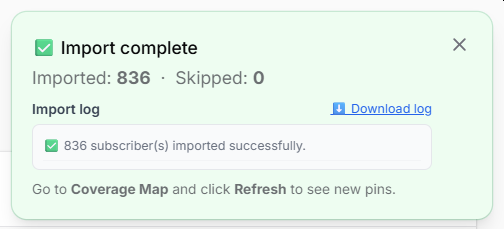
After import, a scrollable log shows the result for each row: imported, skipped (with reason), or failed. The log can be downloaded as a text file.
Coverage Map
The coverage map is the primary workspace in GridVisio. It shows all towers, coverage sectors, subscribers, temp pins, links, drive test data, and analysis overlays for the selected project.
Sidebar → Coverage Map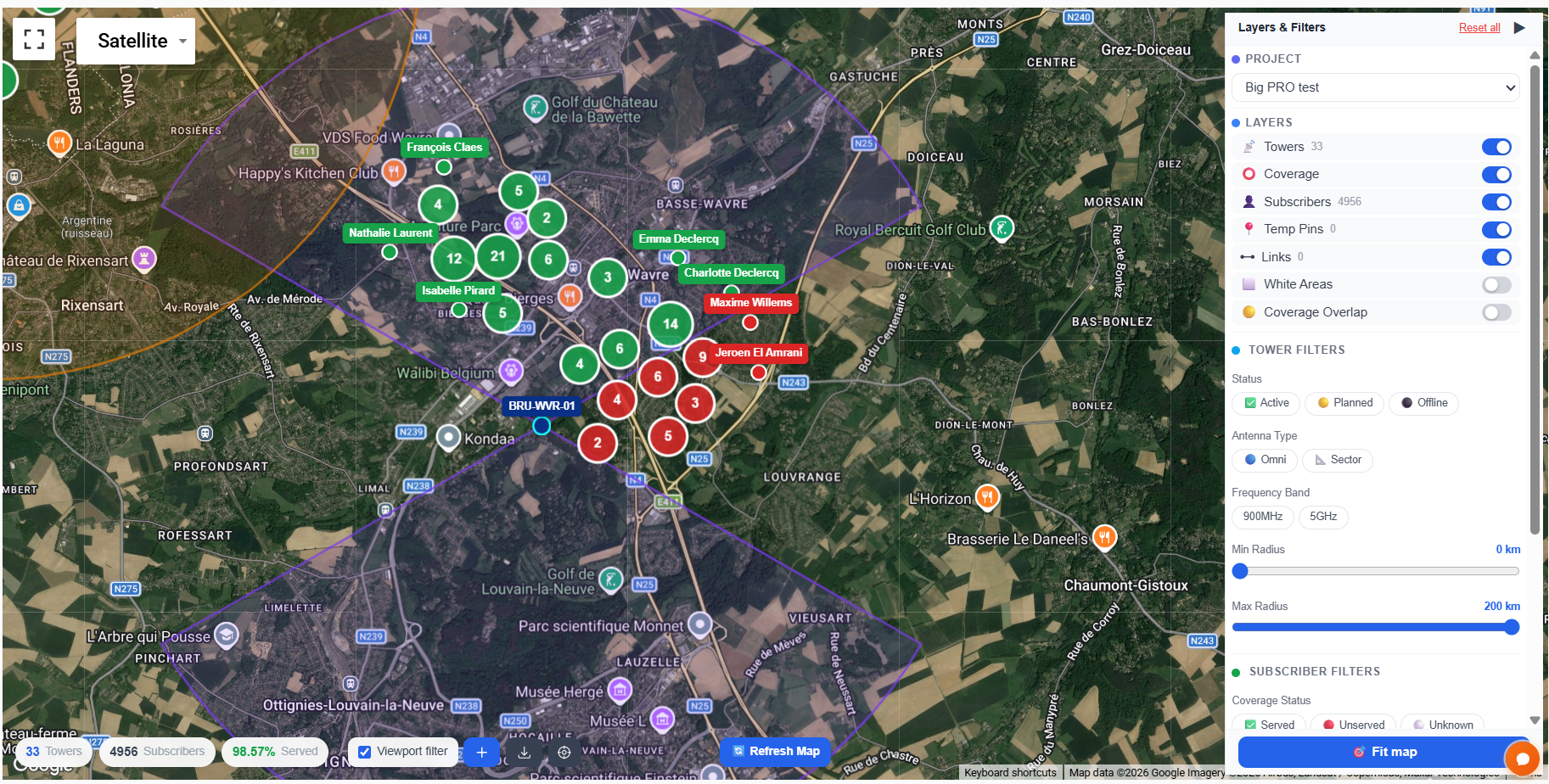
Project selector
The project selector in the Layers & Filters panel (top-right) switches between your projects. The map reloads all data for the selected project.
Map type
Switch between Map, Satellite, Hybrid (satellite + labels), and Terrain using the map type control in the top-right of the map. Your chosen map type is remembered across sessions.
Stats bar
The bottom-left stats bar shows live counts for the currently loaded data: towers, subscribers with served/unserved breakdown, and coverage percentage. These numbers reflect the viewport filter if it is active.
Viewport filter & Refresh Map
By default, GridVisio only loads towers and subscribers that fall within the current visible map area. This keeps performance fast on large projects with thousands of subscribers.
Panning or zooming the map does NOT automatically reload data. This is intentional. After moving the map, the Refresh Map button appears in the toolbar. Click it to load data for the new view.
This is also the key to using subscriber clustering efficiently:
- Zoom into the area you want to inspect
- Click Refresh Map
- Individual subscriber pins replace cluster bubbles for the loaded area
- The stats bar updates to show counts for the current viewport only
Exports (XLSX, KMZ, PDF) respect the viewport filter — only currently loaded towers and subscribers are exported when the filter is active.
Coverage recalculation
Adding, editing, moving or deleting a tower or sector can change which subscribers are covered, so GridVisio re-checks the affected ones. It only re-checks subscribers the change could plausibly reach — near the old and/or new position, within range of the changed sector(s) — not the whole project.
While it runs, a small Recalculating coverage progress indicator appears at the top of the map showing how many subscribers are done. The map stays usable — pan, zoom, measure links, run Rooftop Scan or POP Scan, switch layers. Only the actions that would change towers are paused, because starting a second recalculation on top of a running one isn't supported.
Save now, recalculate later
When you save a tower change that affects coverage, you get two choices:
- Save & Recalculate — saves and immediately re-checks the affected subscribers. Unavailable while another recalculation is already running.
- Save only — saves the change but doesn't re-check anything yet. Use this when editing several towers in one sitting: make all your changes, then recalculate once at the end instead of waiting after each one. Always available, including while a recalculation is running.
Deleting a tower offers the same pair (Delete & Recalculate / Delete only).
Every time you choose to defer, the affected subscribers are remembered and an orange Recalculate N subscribers button appears at the top-left of the map. Click it to bring them all up to date in one pass. The count is kept on the server, so it survives a page reload, a logout, and opening the project on another device — and it covers everyone affected by every deferred change, not just the last one.
Until you run that recalculation, affected subscribers still show their previous coverage status. That's most visible after deleting a tower: its subscribers keep showing as Served even though the tower is gone. Hovering any affected subscriber shows an Out of date notice explaining why, and the orange button is the reminder that the work is still owed — but nothing clears it except running the recalculation.
If a recalculation fails, the affected subscribers stay marked as out of date and the button reappears, so the work is never silently lost.
Quicksearch
A floating search box at the top of the map (positioned to always clear the Layers & Filters panel) finds Towers, Sectors, Subscribers, Links, and Temp Pins by name or address without leaving the map.
Searching
Typing searches automatically once you've entered at least 3 characters (a short debounce after you stop typing). Press Enter to search immediately on 1 or 2 characters instead of waiting until a third.
Results are capped at 20, sorted alphabetically across all types together (a matching tower and a matching subscriber can sit next to each other — results are not grouped by type). If more than 20 items match, a line at the bottom of the list shows the total match count and prompts you to keep typing to narrow it down.
Filtering by type
Prefix the search term with a type qualifier to search only one type of item, the same "operator:value" pattern used by GitHub/Gmail search:
| Qualifier | Example | Searches |
|---|---|---|
t: | t:CHT | Towers and Sectors together (a Sector has no location of its own — it always pans/zooms to its parent tower) |
s: | s:Doe | Subscribers only |
l: | l:Backhaul | Links only |
p: | p:Candidate | Temp Pins only |
The qualifier must be the very first thing typed. No qualifier searches every type, as described above.
Selecting a result
Clicking a result pans and zooms the map to that item's location.
If the viewport filter is on, a result that isn't currently loaded on the map (outside the bounds of the last Refresh Map) is shown with an amber highlight and a "Not in current filtered view" label. Clicking it asks for confirmation before jumping there — panning to it does not trigger a refresh, so the item's marker may still not be visible once you arrive until you click Refresh Map yourself.
Layers & Filters
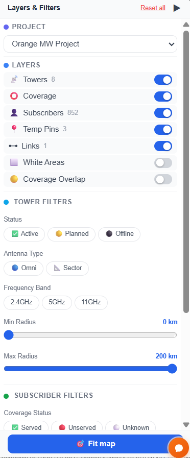
The Layers & Filters panel (toggle with the filter icon top-right) controls what is visible on the map and how data is filtered.
Layer toggles
- Towers — show/hide tower markers and labels
- Coverage — show/hide sector coverage shapes
- Heatmap — show/hide the multi-color RF propagation heatmap for towers currently in view. Disabled until at least one heatmap has been generated for the project — see RF Propagation Heatmap.
- Subscribers — show/hide subscriber markers
- Temp Pins — show/hide hypothetical tower pins and planning pins
- Drive Tests — show/hide drive test signal strength overlays
- White Areas — show/hide unserved subscriber cluster polygons
- Interference Analysis — show/hide sector overlap/interference zone indicators
Redundancy view toggle
A Redundancy view sub-toggle sits directly under the Subscribers layer toggle above (shown only while that layer is on, the same way the Heatmap layer reveals its own data-source sub-toggle). It changes what the subscriber marker colors mean: instead of service status, they show how many separate towers could serve each subscriber, so single points of failure stand out. The status filter chips below switch to match whichever view is active. Pro plans and trials only; see Redundancy View.
Subscriber status filter
Filter subscriber markers by status: served (green), marginal (amber), unserved (red), unknown (gray). Multiple statuses can be selected simultaneously. ("Potential" is a separate manually-flagged layer, not a coverage-status filter value.)
Tower status filter
Filter towers by sector status: active, planned, offline.
Frequency filter
Show only towers that have at least one sector on a specific frequency band. Chips appear for each frequency band present in the project. Multiple frequencies can be selected.
Subscriber clustering
When a project has many subscribers, they are automatically clustered into group bubbles at lower zoom levels. The clustering threshold (below which individual markers are shown) is configurable in Project Settings.
Viewport filter
When enabled, only towers and subscribers within the current map viewport are loaded. A Refresh button appears when you pan the map — click it to reload data for the new viewport. This improves performance on large projects.
Map Tools
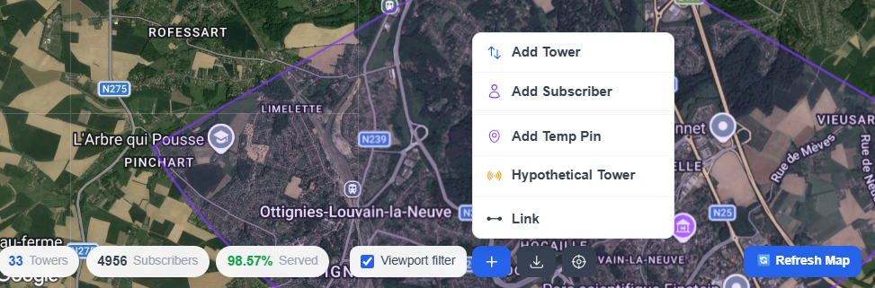
The bottom toolbar contains tools for adding elements and exporting the map.
Adding elements (+ menu)
- Add Tower — click the map to place a new tower at that position. A default sector is created automatically.
- Add Subscriber — click the map to place a new subscriber.
- Add Pin — place a temporary planning pin (hypothetical tower or general marker).
- LoS Link Check — enter link drawing mode to connect two points. Computes distance, bearing, terrain profile with Fresnel zone, LoS status, and free-space path loss. See LoS Link Check for details.
Export menu (▾)
- Export PNG — exports the current map view as a high-resolution PNG image
- PDF Report — generates a formatted PDF report with map image and project statistics
- XLSX Export — exports tower and subscriber data as a structured Excel spreadsheet
- Export KMZ — exports towers, coverage sectors, subscribers, the RF Propagation Heatmap, and saved LoS Checker links as a KMZ file for Google Earth or GIS tools. Towers/sectors/subscribers/heatmap respect the active viewport filter; saved links always export the full project.
- BDC Export — exports subscriber coverage data in Broadband Data Collection format
- BEAD Export — exports in BEAD program format
- Share Map — creates a shareable read-only link to the current map view
Temp Pins & Links
Temporary pins
Temp pins are planning markers that exist on the map without being permanent towers. Two types:
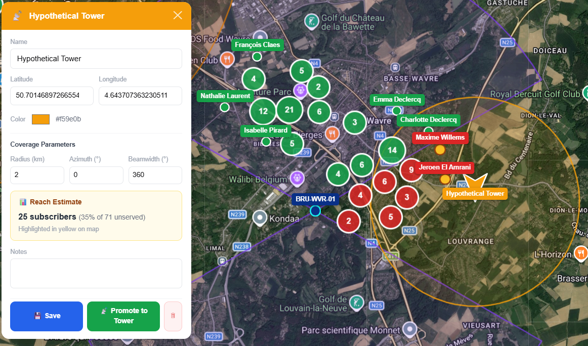
- Hypothetical tower — shows a coverage radius to model a planned deployment. Has azimuth, beamwidth, radius, and frequency fields. Coverage is rendered on the map in real time.
- Planning pin — a general-purpose marker for annotations, potential sites, or reference points.
Pins can be dragged to new positions on the map, or repositioned by editing the latitude/longitude fields in the pin's info panel. Coordinates are validated when you leave the field — a valid position takes effect on the map immediately (the marker moves and any coverage redraws), just like the colour and radius fields. An out-of-range value (latitude outside -90…90 or longitude outside -180…180) shows an error and is not applied; the marker stays where it was until you correct the value.
A new pin lives only in your current session until you click Save to project in its info panel, which persists it to the database (subject to the saved-pin plan limits below). Once saved, further edits — including coordinate changes — are saved automatically. Hypothetical-tower pins can be promoted to real towers from their info panel. Session pins (saved or not) are kept when you refresh the map.
Saved pins (persisted to database across sessions) are limited by plan: Free: 3 saved pins. Trial/Starter: 20 saved pins. Pro: unlimited. Ephemeral pins (not saved to a project) are unlimited on all plans.
Links
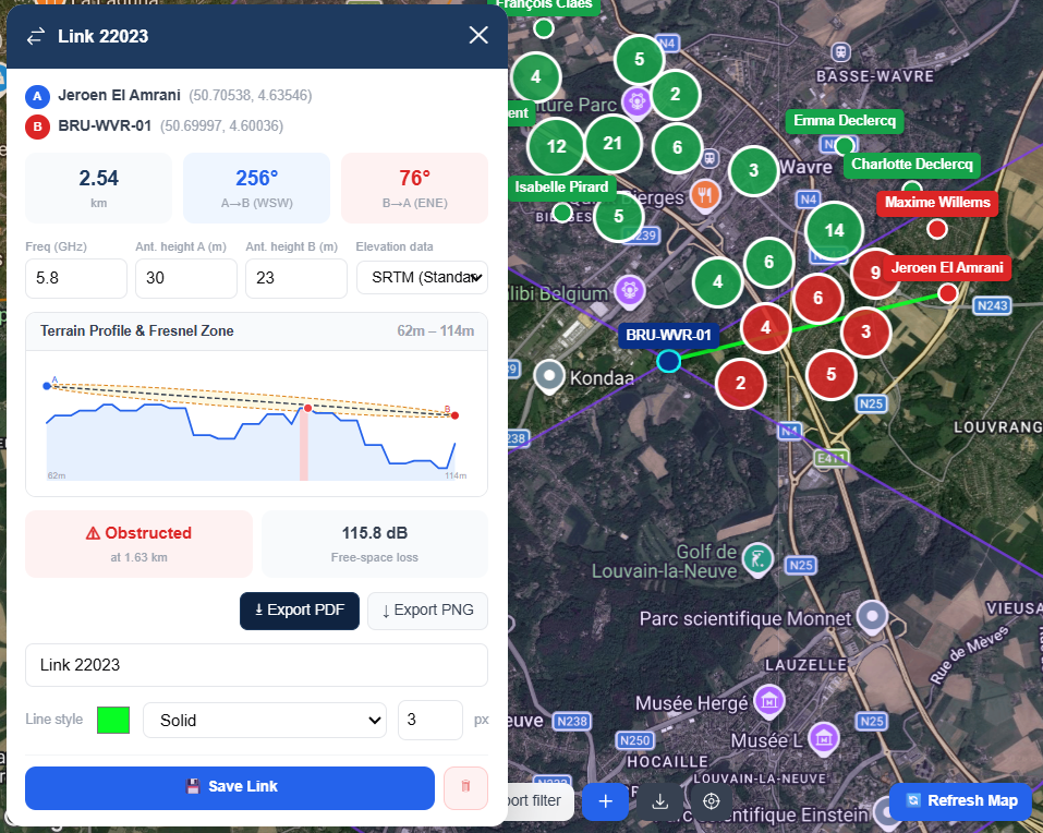
Links connect two points on the map for distance measurement, bearing calculation, and line-of-sight analysis. The full LoS Link Check feature — including Fresnel zone, terrain profile, and PDF export — is documented in the next section.
Ephemeral links (not saved, lost on page refresh): Free: 1. Trial/Starter/Pro: unlimited.
Saved links (persisted to database): Free: 0. Trial: 10. Starter: 50. Pro: unlimited.
LoS Link Check
The LoS Link Check tool measures the line-of-sight path between two map points, renders a terrain cross-section with Fresnel zone overlay, and determines whether the link is clear or obstructed — accounting for estimated vegetation and building height on top of bare-earth elevation, not terrain alone. It is the primary tool for validating antenna placement before deployment.
Map → + menu → LoS Link CheckHow to use
- Click LoS Link Check in the map + menu to enter link drawing mode.
- Click point A on the map (e.g. your tower), then click point B (e.g. a subscriber location).
- The link popover opens automatically with the full analysis.
- Adjust frequency, antenna heights, or elevation source — the terrain profile and Fresnel verdict recompute immediately (pure geometry, no extra fetch). The predicted RSSI number is different: it deliberately does NOT recompute on every keystroke (a real propagation-model spawn, not free) — changed inputs instead dim the RSSI card and show an explicit Re-check button, so the number on screen is never silently wrong, just clearly marked stale until you click it.
Inputs
- Freq (GHz) — link frequency used to calculate Fresnel zone radius and free-space path loss. Default: 5.8 GHz.
- Ant. height A / B (shown in m or ft per your Distance Unit preference) — antenna height above ground at each endpoint, pre-filled automatically and always editable afterward:
- Tower endpoint — GridVisio works out which of the tower's sectors actually covers the direction toward the other endpoint (same geometric test used for subscriber served/unserved status, status-agnostic — a Planned or Offline sector still counts) and pre-fills that sector's antenna height. If more than one sector overlaps that direction, the greater of the two is used by default. If no sector on the tower covers that direction at all — or the tower has none — it falls back to the tower's structure height instead. This applies the same way to a hypothetical tower (planning-only pin), which falls back to the generic 30 m (98.43 ft) default below since hypothetical towers have no per-sector antenna heights to resolve.
- Subscriber endpoint — pre-fills that subscriber's own height field (default 5 m / 16.4 ft).
- Arbitrary map point or temp pin — no record to read a height from, so this falls back to a generic 30 m (98.43 ft) default.
- Sector selector — whenever an endpoint is a tower, a small dropdown appears right under its name showing every sector on that tower that geometrically covers the direction toward the other endpoint — including two or more overlapping sectors (different frequencies/heights pointed the same way), not just the one auto-picked above. Sectors within the tower's declared radius (or extended margin, if your project has that enabled) are listed first, sectors beyond it after — still selectable, never hidden, since checking a link deliberately beyond a sector's declared range is a legitimate use of this tool. Picking a different sector applies its own antenna height and frequency and reruns the full check against it, including a fresh predicted RSSI using that sector's real transmit power and gain. Shown even when only one sector matches, as confirmation of which one GridVisio identified.
- Elevation data — choose between:
- SRTM (Standard) — Open-Elevation API, global coverage, ~30 m resolution. Default.
- Copernicus GLO-30 — Copernicus DEM via OpenTopoData, 30 m resolution, more accurate in mountainous terrain.
- USGS NED 10m (US) — USGS National Elevation Dataset via OpenTopoData, ~10 m resolution, continental US only.
- Propagation model — an ephemeral, session-only override of which model computes the predicted RSSI for this specific link (ITU-R P.1812, ITM/Longley-Rice, or FSPL+ITU-R P.526 — see Choosing a propagation model for how each is selected by default). Pre-filled with whatever the project would normally resolve for this sector's real frequency; changing it never affects any other link or the project default.
Terrain data: LiDAR, land cover & elevation
Every LoS check looks up the most precise terrain data actually available for each point along the path, in priority order, before running the Fresnel check:
- Real measured LiDAR — a real measured surface height, not an estimate, wherever a free public LiDAR dataset covers the location: USGS 3DEP (US), Environment Agency (England), Natural Resources Wales, Scottish Remote Sensing Portal, NRCan HRDEM (Canada), IGN LiDAR HD (France), AHN (Netherlands), IGN/CNIG (Spain), or LINZ (New Zealand). See About the real-measurement LiDAR sources below.
- Land-cover clutter estimate (used wherever LiDAR wasn't used for a point) — estimated land cover (forest, urban, scrub, etc.) with a reference height added on top of bare elevation. Coordinates inside the continental US use USGS NLCD; everywhere else (including Romania/EU) uses ESA WorldCover.
- Bare elevation only — used when neither LiDAR nor land-cover data is available for a point.
The result panel always shows which source was actually used:
- Terrain: USGS 3DEP LiDAR (US) — real measured surface height used along this path. Outside the US, the same wording appears with the actual source that resolved it — e.g. "Environment Agency LiDAR (England, UK)", "AHN LiDAR (Netherlands)" — see below for the full list.
- Terrain: USGS NLCD (US) — NLCD land cover used along this path
- Terrain: ESA WorldCover (Global) — WorldCover land cover used along this path
- Terrain: Mixed sources — different stretches of the same path resolved to different sources (e.g. LiDAR for part of the path, land cover for the rest, right at the edge of 3DEP coverage)
- Terrain: bare elevation only — none of the above had data for this location; the check falls back to bare elevation with no height added, and this is shown explicitly rather than silently degrading
Clutter height estimates (e.g. 15 m for deciduous forest, 25 m for evergreen forest, 8 m for medium-density urban) are reference defaults, tunable by GridVisio admins, with a per-project override layer for WISPs whose region runs taller or shorter than the default — this does not require a code deploy and does not affect any other project.
About the real-measurement LiDAR sources
USGS 3DEP (the 3D Elevation Program) is the USGS's ongoing, multi-year effort to collect airborne LiDAR across the United States — laser pulses fired from a plane that measure the height of whatever they reflect off. Unlike the land-cover estimate above, which infers a typical height for a general category like "forest" or "medium-density urban," LiDAR records the actual height of the real object at that spot: a specific tree, a specific roofline. Every 2 metres along the link, GridVisio takes the highest LiDAR measurement inside that point's own strip of the path — 2 m long and 3 m either side of the line, measured in true metres along the real (geodesic) path — read at the data's full native resolution, never resampled. Where several surveys cover the same spot, the newest one that measured it is used, so a building or tree that is gone isn't kept from an older flight. The result is the real treetop or rooftop there, not a category average. No file formats or point-cloud jargon to know — GridVisio just uses the most precise real measurement available and shows you which kind of data backed the result.
The same real-measurement precision is also available, automatically, from eight other free public government LiDAR programs outside the US: the Environment Agency (England), Natural Resources Wales, the Scottish Remote Sensing Portal, NRCan's HRDEM (Canada), IGN's LiDAR HD (France), AHN (Netherlands), IGN/CNIG (Spain), and LINZ (New Zealand). There's no setting or toggle for any of this and nothing to pick — GridVisio checks USGS 3DEP first, and only if that finds nothing for a location does it check whichever of the other eight actually covers that spot; a WISP outside the US or these other eight countries never sees any difference in behaviour, and a US-only WISP's checks are entirely unaffected by these eight sources existing at all.
This is more precise than the land-cover estimate, but coverage is not yet nationwide for any of the nine sources — each is an ongoing government acquisition project, still expanding year over year, and GridVisio only draws on the freely available public portion of each (no paid data tier, no extra cost passed on to you). Where none of the nine has coverage for a location, the check automatically falls back to the land-cover estimate, then bare elevation, exactly as described above.
Where a real LiDAR measurement exists, the entire path — the terrain profile, the Fresnel/clearance verdict, and the predicted RSSI number, not just the chart — is resolved at a genuine 2 metre grid, the native resolution LiDAR data is actually stored and cached at. Where LiDAR isn't available for any part of the path, the check instead uses a ~30 metre grid, matching the real resolution of the underlying bare-earth/land-cover data itself (SRTM, Copernicus GLO-30, and NLCD/WorldCover are all natively 10–30 m; USGS NED is 10 m) — going any finer there wouldn't add real information, since the source data itself isn't that precise. Point count therefore always scales with the link's actual length and whether LiDAR covers it, never a fixed sample count, so a narrow obstruction like a single tree or roofline can't slip through between two checked points at either resolution. There is one limit on the LiDAR lookup specifically: links longer than 20 km skip the USGS 3DEP lookup entirely (an unusually long distance for the fixed-wireless links GridVisio is built for) and use the land-cover estimate instead. The eight other regional sources have their own length limit instead, based on your plan: 5 km on Free, 10 km on Starter and Trial, 20 km on Pro — long enough for real long-haul WISP backhaul links on Pro. The map's LoS Link Check tool shows an on-chart note whenever LiDAR isn't contributing to a result, explaining whether it's because the link is over the length limit or because no real measurement was found for that specific path. Separately, the LoS Link Check tool itself has an overall maximum link length of 35 km (matching the maximum coverage sector radius elsewhere in GridVisio) — well beyond any realistic single fixed-wireless hop, and rejected with a clear message rather than attempted.
Long links are read the same way as short ones: GridVisio splits the real-data fetch into several pieces requested at once, to keep response times reasonable, but every 2 m point is still answered from the full-resolution data — a long link doesn't get a thinner or coarser profile. A point shows as non-LiDAR only where the surveys genuinely have no measurement there (water, a coverage gap), or where a data source couldn't be read completely in the time available; in that last case the missing stretch uses the land-cover estimate, the result is never saved as final, and the next check of that link fetches it again. A complete profile is kept, so re-checking the same link (in either direction) is near instant. Nothing to configure here.
The terrain source used is also recorded per-tower on any lead the Coverage Widget captures (alongside the existing classification and clearance fields), so the same attribution shown here is visible later in the Lead Inbox and the lead notification email — useful for judging how precise a particular lead's coverage assessment actually was.
Terrain profile & Fresnel zone
- Blue line — bare-earth elevation profile
- Green line — clutter-raised profile (bare elevation + estimated vegetation/building height), layered on top of the blue line, on segments where land-cover data was used
- Orange line — LiDAR-raised profile (real measured surface height from whichever of the seven sources covers this location — see above), layered on top of the blue line, on segments where real LiDAR coverage was used — drawn thicker than the green line since it's the more precise of the two where both could apply
- Dashed line — straight line-of-sight from antenna A to antenna B at their effective ASL heights
- Shaded zone (green = clear, amber = tight) — first Fresnel zone boundary, checked against the most precise profile available at each point (LiDAR, then land cover, then bare elevation), not bare elevation alone. For reliable links, 60% of the first Fresnel zone must be clear at every point along the path.
- Red terrain fill — segments of that profile that penetrate the 60% Fresnel zone clearance
- Red dot — worst obstruction point along the path
- Blue dot (A) / Red dot (B) — antenna positions at effective above-sea-level height
The shaded-zone colour and red fill above show exactly where along the path clearance drops below the 60% line — a per-point view. The overall Clear / Borderline / Obstructed badge below summarises that into one verdict for the whole link, using the worst point on the path.
Click the chart to open a larger, zoomable view — useful for inspecting a specific stretch in detail, especially where LiDAR resolved many more points than the small inline chart can show individually. Scroll/pinch to zoom (toward wherever your cursor/fingers are), drag to pan, or use the on-screen −/+/Fit controls; zooming out floors at the original fit-to-screen view, so there's never empty space around the chart. This is a viewing aid only — Export PDF/PNG always captures the full, un-zoomed chart regardless of what you're currently zoomed into when you export.
Clearance tiers
The Fresnel check computes a continuous clearance value at every point along the path — what fraction of the first Fresnel zone radius is actually clear, expressed as a percentage. The 60% line described above is the pass/fail threshold for that percentage at the single worst point on the path. Rather than collapse that number straight to a binary Clear/Obstructed verdict, the result panel shows one of three tiers:
- Clear (clearance ≥75%) — comfortably above the 60% pass line. A confident clear call.
- ~ Borderline (clearance 40–75%) — close enough to the 60% line that it could go either way depending on real-world conditions and equipment. Treated as inconclusive, not a pass or fail.
- Obstructed (clearance <40%) — well below the line. A confident obstruction call.
The clearance percentage is always shown next to the badge (e.g. "Borderline — 52% Fresnel clearance"), and is saved alongside the existing classification fields on any lead the Coverage Widget captures, so the same tier and percentage are visible later in the Lead Inbox and lead notification email.
Near a path's endpoints the underlying percentage is a ratio against a Fresnel radius that shrinks toward zero, which can swing to extreme, uninformative values (e.g. "-2000%"). Below −100% GridVisio shows "Severely obstructed" instead of the raw number — a display-only clamp; the stored clearance percentage itself is unaffected.
Free-space path loss (FSPL), shown alongside the badge, is the theoretical signal loss over distance assuming a completely unobstructed path — it does not measure or relate to obstruction severity, which is why it's labelled "baseline, no obstruction" rather than placed next to the clearance percentage as if the two were related.
Height Optimizer
On a Borderline or Obstructed result, the clearance badge gains a small Optimize button — on an already-Clear link the same button is still shown, but asks the opposite question. It opens a tool that searches real antenna-height combinations and reports the smallest change that reaches Clear (or, on a Clear link, how much height could be removed and still stay Clear), using the exact same Fresnel engine as the main check — never a separate, less-precise approximation.
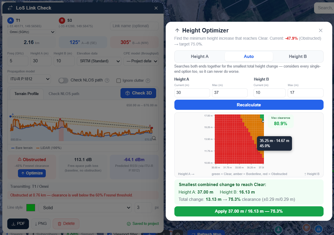
- Height A / Auto / Height B — a 3-way mode toggle, Auto selected by default. Height A/B search one endpoint while holding the other fixed; Auto searches both endpoints together for the combination with the smallest total height change — it considers every single-end option too, so it can never do worse than picking one end by hand.
- Current / Max (or Min) — both endpoints' height fields are always visible and always editable, independent of which mode is selected; only the Max/Min field disables for whichever end the current mode excludes from the search. Current is a draft, not a live view — it starts at the link's real height but only writes back to the actual link when you click Apply, so you can freely explore "what if the other end were mounted higher" without touching the real link until you decide to.
- Auto mode's grid — a colored image (green = Clear, amber = Borderline, red = Obstructed) with Height A along the bottom and Height B along the left, built from a real sweep across both ranges at roughly 20 cm (or 0.5 ft, matching your Distance Unit preference) resolution. Hover any cell for its exact height combination and clearance percentage. A white dot marks the automatic minimum-change recommendation; a small Max Clearance pill above the grid shows the single best percentage found anywhere in it (often higher than the recommendation, since minimizing change deliberately doesn't chase the grid's ceiling).
- Click any cell to apply it instead — the whole point of the grid is seeing every real option, not just the automatic one. Clicking marks that cell (a blue ring) and updates the Apply button to that exact combination.
- Apply — always available, not restricted to a Clear result: the button's own color (green/amber/red) shows which tier you're about to apply, so applying a Borderline or even an Obstructed combination is a deliberate, informed choice rather than a hidden option. Shows the heights and clearance percentage it will set; clicking writes them into Height A/B on the main LoS Checker (marking the RSSI stale for a Re-check, same as editing those fields directly) and closes the Optimizer.
The Height Optimizer doesn't run its own simplified geometry — every number it shows comes from the identical server-side Fresnel calculation (and the identical 75%/40% Clear/Borderline tier thresholds) the main LoS Link Check uses. What changes is which heights are fed into it, swept across a range, instead of the single pair currently set on the link.
NLoS reflection path check
On a Borderline or Obstructed result, a Check NLOS path toggle appears next to the Propagation model selector, and the terrain panel below gains a second tab (labelled with the toggle's own name) alongside Terrain Profile. Switching tabs is purely a view change — it never fetches anything; only the toggle itself does that, and turning it on jumps you straight to its tab so the search is never running invisibly in the background. It searches for one possible reflected signal path — off a nearby flat surface such as a rooftop, water, or open ground — in addition to the direct line already shown above, using the exact same terrain and real-LiDAR precision as the main check (including LiDAR from all seven regional sources, not just the US). It's on-demand only: a real extra terrain fetch runs only when you switch it on, never automatically.
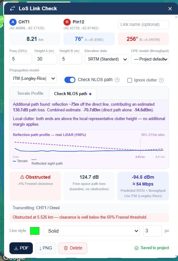
- Additional path found — shows the reflection's lateral offset from the direct line (in metres), the extra path loss it contributes (in dB), and a combined estimate in dBm that accounts for both the direct and reflected paths together, alongside what the direct path alone would predict.
- Reflection path profile — a small terrain chart for the reflected path specifically (tx → reflection point → rx), with its own distance and elevation axes, and the same real-LiDAR-percentage note used on the main terrain profile below.
- No viable additional path found — the search tried several candidate reflection points and none had a genuinely clear path on both legs. This is a real, common result, not an error.
- LiDAR for the reflected path couldn't be completed — where real LiDAR covers the area, each candidate's two legs are checked against the full-resolution LiDAR profile before a reflection is accepted. If that fetch runs out of time or a data source can't be read completely, GridVisio says so instead of guessing; try again (legs already completed are kept, so the retry is faster).
GridVisio tests one candidate specular reflection point at a time (a handful of fixed lateral offsets on either side of the direct line), accepting it only when both legs are independently confirmed clear — not a full multipath or ray-tracing simulation. The direct and reflected path losses are combined as power (non-coherent combining), never as phase — real-world constructive/destructive interference depends on continuously-varying, sub-wavelength path-length differences that no terrain dataset at any resolution can predict; only real hardware measures that. Treat the combined estimate as a plausible best case if that one reflection exists, not a guaranteed number. This is also the honest, geometry-only distinction from NLoS hardware platforms (e.g. those using genuine multipath signal reconstruction, such as Tarana) — GridVisio doesn't model or replicate what that hardware does internally; it surfaces one additional geometric path so you have more information than the direct line alone, nothing more.
Like the predicted RSSI figure, changing frequency, antenna height, or the "Ignore clutter" toggle marks a previously-found reflection result stale (a one-click Re-check banner appears) rather than silently keeping an outdated number on screen — the same banner covers RSSI staleness too, since both go stale from the same input changes.
Local clutter margin (ITU-R P.2108)
Directly below the reflection result, the same tab reports a second, independent number: an additional signal-loss margin from ITU-R P.2108's statistical clutter-loss model, for whichever end of the link (transmitter, receiver, or both) sits below the representative height of its surrounding land cover. This targets a different problem than the single-reflection search above — dense suburban and urban environments rarely fail from one identifiable missing reflector; they fail from many small, unresolvable scatterers (house facades, fences, tree canopy) around a terminal that's embedded in clutter rather than clearing it. No land-cover category or extra terrain fetch is needed — the model's only inputs are frequency, total link distance, and which end(s) qualify, evaluated against the clutter height GridVisio already resolves for that end.
- Neither end embedded — "no additional margin applies." Both antennas already sit above their local clutter height, so this model has nothing to add.
- One or both ends embedded — reports a typical additional loss (dB) and a separate worst-case combined RSSI, using the 90th-percentile figure from the same model. This is a statistical envelope around the whole link, not another arriving signal path — it's never summed into the reflection check's combined RSSI above.
The reflection search above answers "is there one specific, identifiable extra path" — useful where a real reflector exists (a lake, a rooftop, an open field) but useless in dense clutter, where there are too many small scatterers to identify individually. The P.2108 margin answers the opposite kind of question: given that clutter of a certain density surrounds this terminal, what's the statistically expected variability from many unresolvable small effects, without pretending to trace any one of them. Reporting both, separately and clearly labelled, is more honest than trying to combine two different physical claims into one number.
Fade margin (ITU-R P.530)
On a Clear result, the second tab is labelled Fade Margin instead — a different question again: given this direct path is already geometrically clear, how much signal margin (dB) does it need in reserve to keep working through ordinary weather and atmospheric multipath fading, for a given target availability (e.g. 99.9%, 99.99%)? This uses ITU-R P.530's real geoclimatic prediction method (via the same terrain/frequency/distance already known for the link), not another reflection search. There's no separate toggle — since it needs no new terrain fetch, it computes automatically the first time you open the tab.
The reflection check and clutter margin above are both about whether signal reaches the receiver at all, given the terrain. Fade margin is about a link that already has signal, and how much extra headroom to budget so ordinary atmospheric conditions don't intermittently take it down — the standard reliability-engineering question for any already-clear microwave link, independent of the NLoS questions above.
This checkbox is a what-if diagnostic, not a second legitimate verdict — it answers "how much of this obstruction is the land-cover estimate responsible for," not "is this link actually clear." When checked, real USGS 3DEP LiDAR heights (where available) are kept exactly as measured; every other point along the path is recomputed as if it were bare ground, with no land-cover height added. The result panel relabels clearly ("Hypothetical — clutter estimate excluded") so it's never mistaken for the real check, and PDF/PNG export is disabled while it's checked. Same scope as the Equipment selector above: session-only, not saved, no effect on the Coverage Widget or any lead record.
The 60% Fresnel clearance rule, the three-tier classification, and the LiDAR/land-cover-aware terrain check described above are not specific to this tool — the same engine and the same threshold determine served/marginal/unserved on the Coverage Widget and on subscriber RSSI verification, independent of the Equipment selector (which is map-only). USGS 3DEP LiDAR is used automatically the same way everywhere, with no per-feature setting to configure. This includes BEAD export: the same 50-sample, LiDAR-aware prediction that classifies your subscribers is what BEAD reads from — there is no separate, faster, less-precise bulk engine anymore. See BDC & BEAD Export for how that fits into the export flow.
Saving a link
Save Link persists a link's endpoints and styling (colour, line style, width, label) to the project, subject to the link limits noted under Temp Pins & Links above. It also persists every field on the analysis panel — frequency, both antenna heights, elevation source, CPE model, propagation model override, and whether the NLoS reflection toggle was on — so reopening the link later picks up exactly where you left off, without re-entering anything.
Reopening a saved link restores every field above exactly as you last left it, then recomputes the terrain profile, Fresnel verdict, RSSI, and (if it was on) the NLoS reflection check fresh against current terrain — nothing about the computed result itself is cached or frozen, only the input values are. A field falls back to live tower/subscriber resolution only when it was never explicitly set for that link — a link saved before this behaviour existed, or a hypothetical pin with no sector to resolve a height from. The deliberate tradeoff: once a height or frequency has been persisted for a link, reopening it no longer automatically reflects a tower's antenna height changing later — edit the field again (or clear the link and re-draw it) if you want it to pick up a new live value. (Leads captured through the Coverage Widget work differently again — those are frozen historical records, since a lead documents what a visitor was told at the time they submitted the form.)
Export
- Export PNG — downloads the terrain + Fresnel profile as a PNG image
- Export PDF — single-page PDF with link name, endpoint coordinates, antenna heights, bearing, frequency, terrain profile, LoS status, and FSPL. Available on all plans. If the NLoS reflection check was run for this link, its result (offset, reflected loss, combined RSSI, and profile chart) is included too, along with the local clutter margin figure — omitted entirely if the toggle was never switched on, never shown as "not checked."
3D Corridor Check
The 3D Corridor Check renders an actual three-dimensional view of a link's real LiDAR terrain, surrounding buildings, and Fresnel zone — a visual companion to the numbers on the LoS Link Check panel, for the cases where seeing the actual obstruction is clearer than reading a clearance percentage. It fetches the same class of real LiDAR data described above, at a fine grid resolution, and renders it as an explorable 3D scene you can orbit, pan, and walk through.
3D Corridor Check is a Pro plan feature. The 14-day trial gets full access too, with no separate cap. Starter and Free have no access — the Check 3D button is shown but disabled, with a tooltip explaining why.
How to use
- Open a LoS Link Check for the link you want to see in 3D.
- Click Check 3D. A progress bar shows the real LiDAR corridor fetch — this is a separate fetch from the 2D check above, at a finer grid resolution and covering the full width of the corridor, not just the path itself, so it takes longer than the 2D chart appearing.
- Once complete, the 3D scene loads: real terrain height along the whole corridor width, nearby buildings, and the Fresnel zone rings running between the two antennas.
- Switching back to the 2D terrain chart and returning to 3D for the same link is instant — it reuses what was already fetched rather than fetching again. Changing antenna height or frequency in the 2D panel and coming back updates the 3D scene to match, without a fresh fetch either.
What you'll see
- LiDAR terrain columns — the real measured surface, extruded to height and coloured on a relative scale (greener = lower, orange = higher, relative to the rest of the current scene, not an absolute colour key) — the same real measurement described in About the real-measurement LiDAR sources above, just shown as terrain instead of a 2D chart. A column outlined in red marks a cell that intrudes into the first Fresnel zone.
- Buildings — nearby building footprints (from OpenStreetMap) extruded to their real height, drawn semi-transparent so the LiDAR detail underneath remains visible rather than being hidden behind a solid grey box. Where a building is mapped with individually-tiered sections (OSM's
building:partdata — common for setback/stepped towers), each tier is drawn at its own real height and starting elevation instead of one flat box for the whole structure. - Fresnel zone rings — a series of rings along the path showing the first Fresnel zone's true radius at each point, exactly matching the geometry the 2D clearance check itself uses.
- Clearance badge — the same Clear / Borderline / Obstructed verdict and clearance percentage as the 2D panel's badge (identical 75%/40% tier thresholds), computed from the same real terrain now visible around it, and using the same authoritative ground reference at each antenna endpoint as the 2D check.
Navigating the scene
The toolbar along the top of the 3D view is split into two groups: an animation group on the left (flythrough + recording controls) and a navigation group on the right (fixed camera jumps and view controls), separated by a thin divider.
- Orbit / pan / zoom / rotate — drag to orbit, scroll to zoom, right-click-drag (or two-finger drag) to pan, the same controls as the main map.
- A→B / B→A — flies the camera along the link from one end to the other, following the real terrain height. Clicking either button always restarts the flight from that end's own starting position, even if a flight in the other direction was already in progress or paused.
- Play / Pause (the flight itself) — appears once a flight has started. Dragging, zooming, or rotating the map while a flight is playing pauses it in place rather than cancelling it — the camera stays exactly where you left it, and the flight remembers how far along the line it had gotten. Clicking Play resumes from that same point, continuing in whatever direction/zoom you last set the camera to — so you can pause mid-flight, look around or line up a better angle, and then carry on rather than starting over. The icon is a paper airplane while playing (click to pause) and the same airplane with a red diagonal line through it while paused (click to resume).
- A-end / B-end — jump the camera straight to either antenna. Always a full reset, not a pause — it cancels any in-progress or paused flight.
- Click anywhere in the 3D scene — on either the LiDAR terrain or a building — pans the 2D map underneath to that exact real-world ground point. This uses a real depth-buffer read, not a naive click-ray projection, so it stays precise even when you're viewing a surface from an angle rather than straight down (clicking the visible side of a tall column or building still resolves to its true position, not wherever the click ray happens to continue to). Useful for identifying what a specific feature in the 3D view actually is on the map — a street, a specific building — without leaving the 3D check.
- Fullscreen — expands the 3D view to fill the available space.
- Back to 2D — returns to the LoS Link Check panel without losing the 3D scene; reopening Check 3D for the same link picks up instantly (see above).
Recording a flythrough video
Next to the flight's own Play/Pause button, a separate light-grey pill holds two more controls — a Record button (a red dot) and a Stop button (a square, greyed out until a recording is running). These capture exactly what's on screen — terrain, buildings, Fresnel zone, and camera movement — as a video file you can save and share, e.g. to show a customer or colleague what a link actually looks like rather than sending a static screenshot.
- Recording is independent of the flight. You can record while manually orbiting the scene with no flight running at all, keep recording through a flight's own pause, or pause just the recording while a flight keeps playing underneath — the two controls never affect each other. Pausing a recording (via the same Record button, which switches to a pause icon while recording) and resuming it later produces one continuous video — the paused time simply isn't in the file, rather than starting a new recording each time.
- Clicking Stop finalizes the recording and immediately offers it to save, straight from the browser. Reaching the end of a flight naturally does the same, with no extra click needed.
- Switching away while recording asks first. Toggling Fullscreen, or clicking A→B/B→A/A-end/B-end, would change the view in a way that can't be undone mid-recording — each of these prompts a confirmation ("This will stop your current recording — continue?") before proceeding, so a recording is never lost by an accidental click. Choosing to continue stops the recording and offers it for saving, same as clicking Stop; choosing not to leaves the recording running untouched.
- Local to your browser only. Recording happens entirely on your own device — nothing is uploaded or stored on GridVisio's servers. The file downloads in WebM format (playable in Chrome, Firefox, and Edge, and most video players and editing tools) once you stop it.
Video recording relies on a browser capability that Safari (on both Mac and iPhone/iPad) does not currently support. In Safari, the Record button is shown greyed out with a tooltip explaining why, rather than failing silently if clicked — everything else in the 3D Corridor Check, including the flythrough itself, works the same as in any other browser.
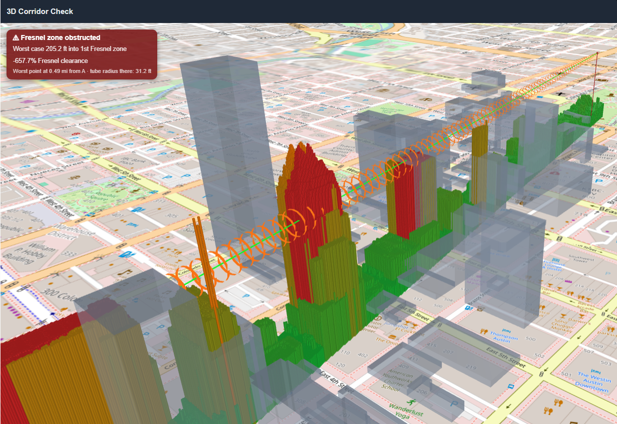
A tall or dense building would otherwise render as one solid box hiding the more detailed LiDAR terrain directly beneath it. Drawing buildings semi-transparent keeps that real terrain detail visible at the same time, rather than making you toggle buildings off to see it.
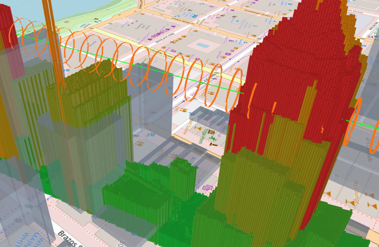
On the 2D map, at the same time
Opening Check 3D doesn't only draw the 3D scene — it also overlays two things directly on the real satellite map, so the corridor's shape and any obstruction are visible even while you're not looking at the 3D view:
- The true Fresnel zone shape — a blue tapering outline (narrow at each antenna, widest at the path's midpoint — the real first Fresnel zone shape, not a plain rectangle) appears on the map the instant you click Check 3D, from pure geometry, before any LiDAR data has even loaded. It's redrawn slightly once the real fetch completes, using the corridor's actual (occasionally capped) width.
- Obstruction markers — once clearance is computed, red "✕" markers appear on the map at the worst obstruction point along each of 20 equal segments of the path (the single worst point per segment, not every intruding cell, to keep the map readable) — the same intrusions drawn as solid red columns in the 3D scene.
The blue outline and red obstruction markers are not tied to the 3D view being open — they stay on the map while you're looking at the plain 2D LoS Link Check panel for the same link, so you can see exactly where a check found trouble without reopening the 3D view. They're cleared only when you select a different link (or close the LoS Link Check popover entirely).
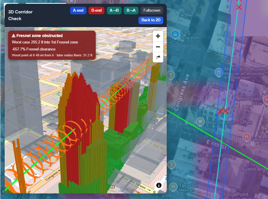
The 3D corridor fetch covers the full width of the corridor at a fine grid resolution, not just a thin line along the path, so it's a heavier fetch than the 2D terrain profile above — a link near the maximum 15 km length can take several minutes the first time. If a fetch fails or times out, a Retry button appears in place of the error message to start it again without leaving the panel.
Drive Tests
Drive test data shows signal strength measurements collected while driving through a coverage area. It is overlaid on the map as coloured dots or a heatmap.
Map → Layers panel → Drive Tests → ImportDrive test import requires a Starter or Pro plan.
Import format
Drive test files are imported as CSV with columns:
lat, lng, signal_dbm, timestamp (optional)Signal strength is displayed on a colour scale from red (weak, e.g. −90 dBm) to green (strong, e.g. −60 dBm).
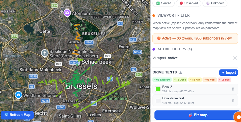
Coordinate Converter
The coordinate converter is a map tool for converting between WGS84 decimal coordinates (latitude/longitude) and Belgian Lambert projected coordinates (X/Y easting/northing) — and, since it's the fastest way to get a specific location onto the map, for looking up an address directly. Available to all plans.
Map toolbar → target icon button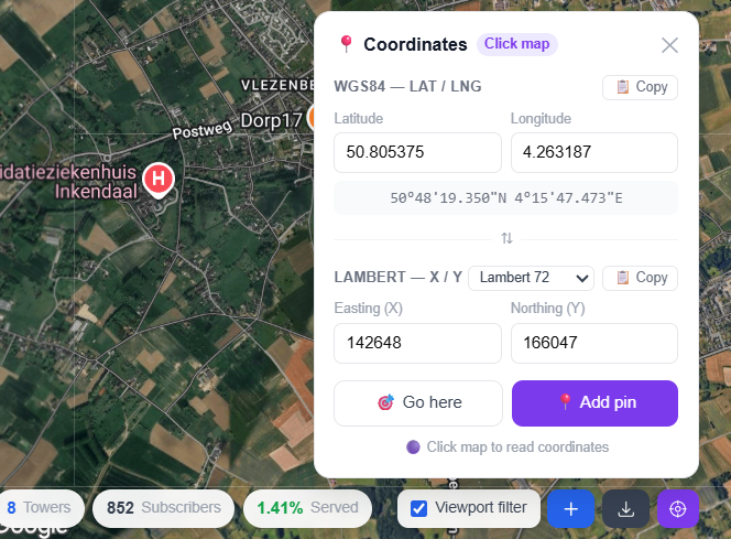
How to use
- 1Open the converter
Click the target icon () in the bottom toolbar. The converter popover opens.
- 2Search an address (optional)
Type an address into the Address field at the top and click Go — the map jumps straight to it and every coordinate field below fills in automatically. This is the fastest way to get a specific address onto the map without knowing its coordinates up front.
- 3Or activate click mode
Click the button again to activate crosshair mode (button turns purple). Click anywhere on the map to populate the coordinates automatically.
- 4Enter or edit coordinates
Type in any field — lat/lng or Lambert X/Y. All other fields update automatically. The DMS (degrees, minutes, seconds) display updates in real time below the lat/lng fields.
- 5Choose Lambert system
Select Lambert 72 (EPSG:31370), Lambert 2008 (EPSG:3812), or Lambert 2005 (EPSG:3447) from the dropdown. Your choice is remembered for the session.
- 6Copy or navigate
Click Copy next to WGS84 to copy "lat, lng" to clipboard. Click Copy next to Lambert to copy "X, Y". Click Go here to pan the map to the coordinates. Click Add pin to create a temp pin at that location — useful as a target for POP Scan when you want to check line of sight to an address rather than a spot you clicked by eye.
Address search uses OpenStreetMap's Nominatim geocoding service, called directly from your browser — no API key required, same service the embeddable Coverage Widget's own address field uses.
Conversion uses the Lambert Conformal Conic (LCC) projection formulas implemented in pure JavaScript — no external library required. Lambert 72 (BD72 datum) includes the WGS84↔BD72 datum shift for ~1–5m accuracy. Lambert 2008 and 2005 use the ETRS89 datum which is coincident with WGS84 for Belgium. Lambert X/Y values are integers (metre precision), which is sufficient for WISP field work.
Supported systems
- Lambert 72 (EPSG:31370) — legacy Belgian standard, widely used in existing infrastructure documentation, Ericsson/Nokia site databases, and topographic maps
- Lambert 2008 (EPSG:3812) — modern replacement for Lambert 72, used in new Belgian government datasets
- Lambert 2005 (EPSG:3447) — intermediate system, superseded by Lambert 2008
White Area Detection
White area detection identifies geographic clusters of unserved or unknown subscribers — areas where coverage is absent despite apparent demand. Results are shown as shaded polygons on the map.
Map → Layers panel → White Areas → toggle onWhite area detection requires a Starter or Pro plan.
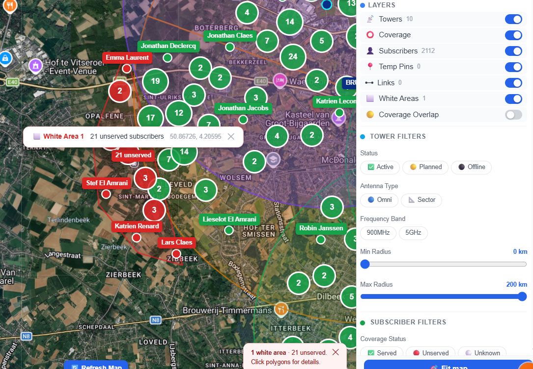
White areas are detected using the DBSCAN (Density-Based Spatial Clustering of Applications with Noise) algorithm. DBSCAN groups points that are close together (within epsilon km) and have enough neighbors (at least min_points subscribers). Points that don't belong to any cluster are classified as noise and ignored. After clustering, a convex hull is computed around each cluster and buffered outward by a configurable distance for visual clarity. DBSCAN is well-suited for this use case because it finds arbitrarily shaped clusters and doesn't require specifying the number of clusters in advance.
Configuration (Project Settings)
- Cluster radius (ε) — maximum distance between two subscribers to be considered neighbours. Default: 2.0 km
- Minimum subscribers — minimum cluster size to form a white area. Default: 3
- Hull buffer — outward padding on polygon edges. Default: 0.3 km
These parameters can be tuned in Project Settings → White Area Detection.
Viewport filtering
White area detection respects the viewport filter. When the filter is active, only subscribers within the current map bounds are analysed.
Interference Analysis
Identifies sectors from different towers whose coverage areas could realistically interfere with each other, and — on Pro plans and trials — computes a real, terrain-and-propagation-backed carrier-to-interference number for the worst point in each zone, not just a geometric "these shapes intersect" flag.
Map → Layers panel → Interference Analysis → toggle onThe base overlap layer (which sectors are in a candidate zone, and a rough estimated severity) requires a Starter or Pro plan. The real per-zone C/(I+N) grid — the colored mini-heatmap and the exact dB number in every popover — requires a Pro plan or trial, the same tier as the RF Heatmap and LoS Link Check's predicted RSSI.
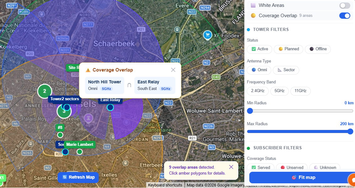
How a zone is found
For every pair of sectors on different towers, the system first checks whether they could realistically interfere at all:
- Co-channel — the two sectors' configured frequencies are identical. Always checked, regardless of whether either sector has a linked equipment preset.
- Adjacent-channel — different frequencies whose channels spectrally overlap, given known channel bandwidth (from a linked equipment preset) on at least one side. Where only one side's bandwidth is known, the system still proves overlap using that side's known channel span reaching the other sector's exact frequency — a provable lower bound, never a guess. Where neither side's bandwidth is known, the pair is not checked (no assumed bandwidth is ever substituted — a real project mixes equipment from many vendors, and guessing one bandwidth for unmodeled gear would misrepresent it as confidently as the modeled sectors).
Pairs are excluded entirely if both sectors are on the same tower — co-located/"co-site" interference is a real, different phenomenon (near-field antenna-to-antenna coupling, not the terrain-based path loss this feature otherwise models) and isn't covered by this analysis.
Sector status: both active and planned sectors are checked — this analysis exists to catch a conflict before it goes live, not just after, so a not-yet-built sector's configured frequency/power is treated as real as an active one's. Offline sectors are excluded (typically decommissioned or dead gear, not "coming soon"). Any zone involving a non-active sector shows that sector's status everywhere it's named — the zone list, the summary popover, and the grid-cell contributor breakdown — so a planned-sector conflict is never mistaken for a live one.
Qualifying, geometrically-overlapping pairs are clustered into zones — a zone can involve more than 2 sectors where several pairwise overlaps connect, and the map list is sorted worst-estimated-severity first so the areas most worth checking on a dense network surface at the top. Clicking a zone (in the list or on the map) zooms and centers the map so the zone's real overlap area fills roughly the middle half of the screen — needed because a real overlap area can be a small sliver that's invisible at whatever zoom you were already at, especially on a dense multi-sector project.
Clicking a zone (in the list or on the map) computes a real grid across the zone's actual overlap area, built from the contributing sectors' own RF Heatmaps: each sector's predicted signal at a grid point is its heatmap's value there — the same terrain/LiDAR-aware propagation (ITU-R P.1812 / ITM / FSPL+ITU-R P.526) and link budget the heatmap layer shows, so the two always agree. The grid is as fine as the finest contributing heatmap, so no heatmap detail is skipped. Every sector in the zone needs a generated heatmap first — if any is missing (or still generating, or failed), clicking the zone tells you which ones; generate them, then open the zone again. Sectors whose frequency no propagation model covers can't have a heatmap and are left out, as before. On a trial, heatmaps cover only part of a large sector's radius, so a sector contributes only where its heatmap was computed. At every point, every sector that geometrically reaches it is evaluated: the strongest predicted signal is the carrier, and every other co-channel or adjacent-channel sector's signal is summed (in linear power, not dB) into the interference total — a point with three overlapping same-frequency sectors sums all three, not just the worst pair. A real thermal noise floor is added using the Johnson–Nyquist formula (-174 dBm/Hz + 10·log₁₀(bandwidth) + noise figure, the same textbook default CloudRF's own published methodology falls back to), from the carrier's linked equipment preset where known. Adjacent-channel contributions are reduced by a fixed 35dB rejection factor, sourced from published 802.11-class 5GHz (20MHz channel) adjacent-channel-rejection specifications — the actual chipset family most WISP AP/CPE radios are built on. This computation only runs once per zone (not eagerly for an entire project) and is cached until a contributing sector, its tower's position, its linked equipment, or one of its heatmaps changes. A very large zone may be computed on somewhat coarser cells than its heatmaps — the zone's popover says so when that happens.
Severity thresholds
Each grid point is classified clean / degraded / severe by its computed C/(I+N) in dB, using whichever threshold is more specific:
- Equipment-derived — where the carrier sector's linked equipment preset publishes a per-modulation required SNR (e.g. Cambium's 450 platform), "clean" is the requirement for its highest modulation tier (enough margin for full-rate operation) and "severe" is the requirement for its lowest tier (below this, not even the most robust modulation is usable).
- Fallback — where no such equipment data exists, ≥18dB is treated as clean and <12dB as severe, sourced from published cellular/point-to-multipoint carrier-to-interference planning literature (not CloudRF's commonly-cited J/S tiers, which are tuned for a jamming-assessment context rather than ordinary link-budget planning and would misrepresent what's actually acceptable for a WISP link).
The base zone polygons are colored by a cheap, free-space-only estimate the moment the layer loads — useful for triage, not the final word. Clicking a zone replaces that flat color with a real graded grid once computed; hovering an individual cell shows its C/(I+N) and dominant interferer, and clicking a cell opens the full contributor breakdown (every sector reaching that point, with its share of the total interference power — a share marked with an asterisk means it's a proven lower bound because that sector's real channel bandwidth isn't known).
RF Propagation Heatmap
The heatmap predicts signal strength across the area around a sector — not just along one line like LoS Link Check, but as a continuous grid. It answers "roughly how strong is the signal here" for every point within a sector's radius, not just "is this one specific spot in line of sight."
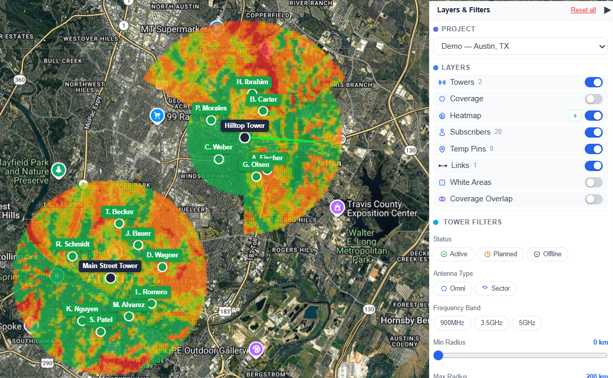
RF propagation heatmaps are a Pro plan feature. The 14-day trial also gets access, capped to a flat 5 km generation radius — enough to see the feature genuinely working, not a like-for-like preview of the Pro experience. Starter and Free have no access.
Pro's generation radius: up to ~22 km, area-based rather than one flat number
A sector's real generation cost tracks its query area — radius combined with beamwidth, capped against a real, measured safe-area ceiling — not radius alone: a narrow, focused sector covers far less real ground than a wide or omnidirectional one at the same radius, so it can safely reach much further out. Pro's own ceiling reflects that directly: the narrower a sector's beamwidth, the further its heatmap can reach, up to ~22 km at the narrowest.
Some real examples of beamwidth/radius combinations at that safe-area ceiling:
| Beamwidth | Max generation radius |
|---|---|
| 3° (narrow, focused) | ~22 km |
| 10° | ~21 km |
| 45° | ~18–19 km |
| 90° | ~14–15 km |
| 360° (omnidirectional) | ~9–10 km |
A sector configured with a radius beyond its own beamwidth's ceiling still generates — coverage is computed out to that ceiling, not rejected outright; the remainder of the configured radius simply isn't included in that generation.
This area-based ceiling currently applies to towers within the continental US. Towers in Canada or any of the other seven supported LiDAR regions (England, Wales, Scotland, France, Netherlands, Spain, New Zealand) keep a flat 15 km ceiling for now, regardless of beamwidth — that number hasn't yet been measured against each region's own real data the way the US figures above have.
What it actually computes
Each generated heatmap is one computed grid of predicted signal strength (dBm), using this project's configured propagation model(s) to predict path loss to every point in the grid. It uses the same real terrain elevation and land-cover (vegetation/building height) data as LoS Link Check, plus each sector's transmit power and antenna gain, to convert that path loss into an absolute signal strength.
Grid resolution adapts to each sector automatically — a small or narrow (directional) sector gets a finer grid than a large, wide-coverage one, so detail isn't wasted where it isn't needed and isn't sacrificed where it is. This happens without any setting to configure; every generated heatmap picks the finest resolution that's safe for that specific sector.
Choosing a propagation model
GridVisio supports three propagation models, each with a different valid frequency range — no single model covers every WISP frequency band, so relying on one alone left real gaps (an 11 GHz backhaul sector or a 60 GHz mmWave link would previously fail to compute at all).
ITU-R P.1812
30 MHz–6 GHz. An internationally standardised, ITU-published point-to-area model built specifically for shorter terrestrial links like fixed wireless — the most accurate choice for the sub-6GHz access frequencies that make up most of a WISP's subscriber-facing traffic, and the default first-tried model.
ITM (Longley-Rice)
20 MHz–20 GHz. The classic NTIA/FCC-origin model, with the most US regulatory precedent — extends coverage into microwave-backhaul frequencies (e.g. 11 GHz) P.1812 can't reach.
FSPL + ITU-R P.526
30 MHz–100 GHz. Free-space path loss plus ITU-R P.526 knife-edge diffraction — the catch-all for true mmWave links (24/60 GHz) neither of the other two models supports.
Every project defaults to all three, in that order (P.1812 first for accuracy on the common case, automatically extending into ITM's and then FSPL+P.526's wider domains as needed) — configurable in Project Settings → RF Heatmap → Model Selection, where you can disable a model entirely or reorder the preference. A single sector can also pin one specific model of its own (in the sector's edit form, next to Colour) — if that model can't cover the sector's own frequency, resolution automatically falls back to the project's order instead of failing. Reordering so a wider-domain model sits before a narrower one it fully covers makes the narrower one unreachable — Project Settings flags this with a non-blocking warning if it happens.
Every computed result — heatmap, LoS Link Check, subscriber classification, BEAD export — records which model actually ran, shown as a small badge/tag next to the number.
Same honest framing as the LoS Link Check's clearance tiers: every one of these models is a well-validated, real-world propagation model, but each is still a statistical prediction from terrain and land-cover estimates — not a measurement. Real signal strength at any given point can differ from the prediction due to local conditions the model can't see (a single building, foliage density at the exact spot, multipath effects, equipment variance). Treat the heatmap as a planning aid for where to focus a closer look (e.g. a real LoS Link Check or a site visit), not as a substitute for one.
Antenna tilt (mechanical or electrical downtilt) is not modelled — every point within a sector's azimuth/beamwidth wedge is treated as receiving that sector's full antenna gain, regardless of elevation angle. This is a deliberate scope decision for now, not an oversight.
Unlike the Coverage Widget, POP Scan, Rooftop Scan, and Classification's RSSI/throughput verification — which all skip Planned and Offline sectors as live candidates (see sector Status for the full breakdown of which policy each tool follows) — heatmap generation includes sectors of every status, including Planned and Offline. This is an internal planning tool, not a public- or subscriber-facing claim, so previewing a Planned sector's predicted footprint before it's actually built is exactly the point.
Generating a heatmap
A heatmap can be generated for a single sector, a whole tower (all its sectors), or an entire project (all towers). Generation runs in the background — it does not block the page, and you don't need to keep it open while it runs.
- Single sector / whole tower — click a tower marker to open its detail popover (not the edit modal), then use the Generate Heatmap button on a sector card, or Heatmap in the popover's footer for all of that tower's sectors.
- Entire project — the + button next to the Heatmap row in the map's Layers panel, or the Generate Heatmap button on the project view page.
Every trigger opens a confirmation explaining what's about to happen and roughly how long it can take before actually starting — nothing is generated without that explicit confirmation.

Checking status
Sidebar → Network → Heatmap JobsEach request appears as one row showing its scope (sector / tower / project), status (Queued / Running / Done / Failed / Done with errors), and timestamps. A tower or project-wide request fans out into one underlying computation per sector — shown as a compact per-sector status list ( / / ) on that same row, so a request covering several sectors can finish with some done and others failed without losing the ones that succeeded.
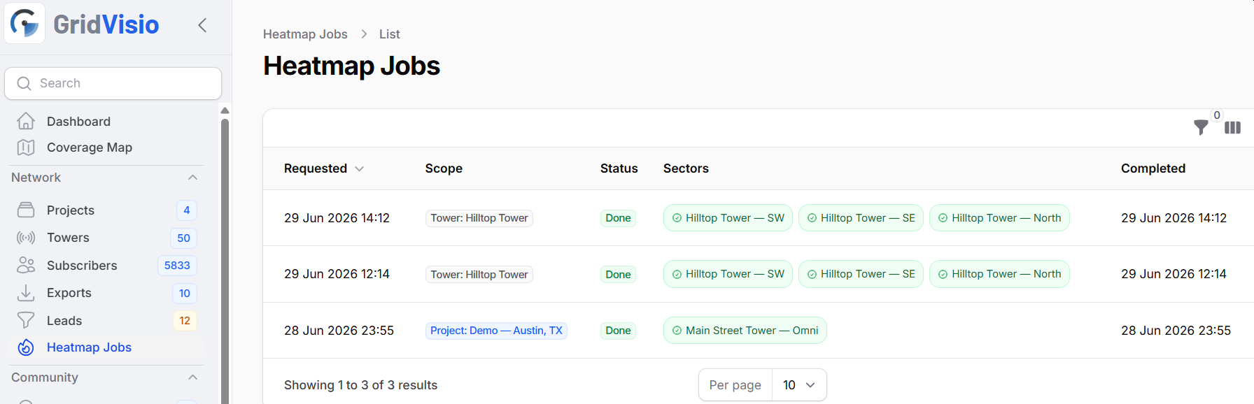
Two display modes, one underlying grid
Both modes render from the exact same computed grid for a given sector — generating a heatmap is never done twice for the same data, only the threshold/colours applied at display time differ, configurable in Project Settings. The internal map's Heatmap layer also has its own live opacity slider (Layers panel, next to the layer toggle) — session-only, adjusts instantly with no re-fetch, and never touches Project Settings; it just starts from that project's saved percentage the first time a heatmap loads each session. The Coverage layer (sector wedge/circle shapes) has the same style of slider right below it, for the same reason — it just has no Project Settings value behind it, so it always starts at a fixed 25%.
Multi-color (internal)
A togglable layer on the main Coverage Map (Layers panel), off by default. Shows configurable signal-strength bands in colour across the area. Viewport-filtered the same way towers/subscribers already are — filter the map to one tower to see just its heatmap.
Single-color (public)
A "covered / not covered" view against one configurable dBm threshold, for the public/embeddable Shared Maps link — not a layer on the internal map. Enable it when creating or editing a share link.

Turning the Heatmap layer on or off only displays an already-generated heatmap if one exists — it never starts a new generation by itself. The toggle is disabled entirely until at least one heatmap has been generated for the project. A one-time explainer covers this the first time you turn the layer on.
Link budget
Every propagation model above only predicts path loss from geometry and terrain — converting that into an absolute signal strength (dBm) needs a simple link-budget calculation on top, identical regardless of which model computed the loss: signal = TX power + antenna gain − cable loss − path loss + CPE gain. TX power and antenna gain are real, sector-specific hardware values (see Sector fields); cable loss and CPE gain are project-wide assumptions about a typical subscriber radio, configurable in Project Settings, since there's no real subscriber to read a value from for a hypothetical grid cell.
Rooftop Scan
Rooftop Scan answers a different question than a single LoS Link Check: not "is this one exact spot clear," but "where on this specific building would a dish actually get the best signal." Click a rooftop on the map and it automatically detects the building's footprint, scans a ring of realistic mounting points around its edge against your chosen tower, and surfaces the best one it found — instead of you guessing a spot and checking it by hand.
Rooftop Scan is a Pro plan feature. The 14-day trial gets full access too, with no separate cap. Starter and Free have no access.
How it works
- Open the map's + menu and choose Rooftop Scan, then click a building on the map.
- GridVisio looks up that building's real footprint from OpenStreetMap first; if OSM has no traced outline there, it falls back to detecting the roof directly from LiDAR surface data. Either way, you see the detected outline over the satellite basemap and can confirm or adjust it before scanning.
- Pick the tower/sector to test against, then run the scan. Every sector — on any tower — that geometrically reaches the rooftop is listed as its own candidate, including two or more overlapping sectors on the same tower (e.g. different frequencies pointed the same direction), not collapsed down to one option per tower.
- The scan runs in the background — you don't need to keep the panel open while it works — and returns a ring of candidate points around the roof's edge, each with its own predicted signal strength and Fresnel clearance, plus a highlighted Best point: the candidate with the strongest realistic signal.
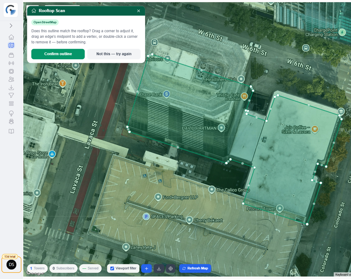
Every candidate point's Fresnel profile is computed the exact same way a manual LoS Link Check line between the tower and that point would be — the same dense, real-LiDAR-merged terrain profile, not a coarser approximation. A Rooftop Scan result and a LoS Link Check drawn to the same point are expected to agree.
The results panel's Terrain source for the best point is the same breakdown a LoS Link Check shows for that link — for example "92% LiDAR (Canada) · 8% WorldCover" — so you can see how much of the path was real measured LiDAR and from which source. The scan only reports LiDAR when real LiDAR was actually read; if it couldn't be, it says so.
From a scan result
Clicking any candidate point (including the Best point) opens the same result popover the map's other LoS tools use — predicted signal strength, Fresnel clearance status, surface elevation source, and the antenna height the scan assumed. A LoS Check button on that popover opens the full interactive LoS Link Check panel pre-filled with that exact point, if you want to explore antenna heights, frequency, or CPE equipment beyond what the scan itself assumed.
Antenna height. Like the LoS Link Check, heights are measured from the ground. At each candidate point the scan places the CPE antenna 1 m above that point's own roof surface — the roof's height above ground plus 1 m — so it never sits below the roof. The popover shows that height above ground, and the LoS Check button pre-fills it, so the LoS Link Check starts from the same antenna position the scan scored.
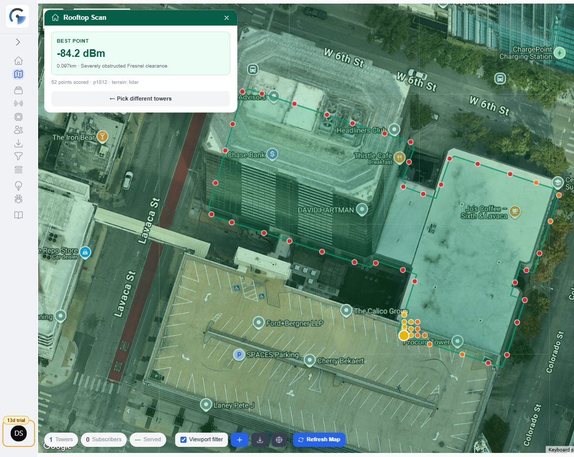
Like every other prediction in GridVisio, Rooftop Scan is only as good as the underlying terrain/LiDAR data for that location — real-world factors a remote scan can't see (a chimney, an HVAC unit, nearby vegetation that's grown since the data was captured) can still affect an actual installation. Use it to narrow down where on a roof to look, not as a replacement for a site visit before committing to a mount point.
POP Scan
POP Scan answers a different question than a single LoS Link Check: not "is this one specific tower clear to this point," but "which of my POPs — Points of Presence, i.e. towers — can reach this spot, how well, and how high would the antenna need to be?" Switch it on, then simply click around the map — a roof, a subscriber, an existing tower, a pin. Every click checks that point against every tower/sector whose coverage reaches it and shows the results in a compact table right at the click. Click another spot nearby and the table updates for the new spot.
POP Scan is a Pro plan feature. The 14-day trial gets full access too, with no separate cap. Starter and Free have no access.
How it works
- Open the map's + menu and choose POP Scan. A small control panel appears at the bottom left and the cursor becomes a crosshair. POP Scan stays on until you click Exit.
- Click any point — a roof, a plain spot, an existing tower, a subscriber, or a pin (including one dropped from the Coordinate Converter's address lookup). A results table opens at the clicked point and fills in tower by tower; a line is drawn from each tower to the point, colored by its Fresnel tier.
- Click somewhere else to check that spot instead — no confirmation steps. The first click in an area reads the LiDAR around it, which can take a while (typically tens of seconds, more for a long link or a slow data source); clicks within about 50 m of it afterwards are answered much faster from the data already read.
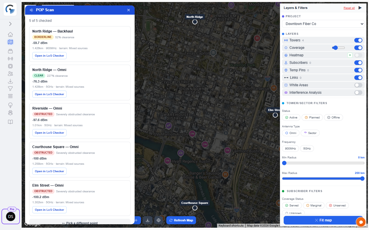
Height above ground or above the roof
The control panel sets the antenna height at the clicked point, with a slider and a Ground / Surface (roof) toggle:
- Surface (roof) (the default, 2 m): the height above whatever surface LiDAR measured at the point — typically a roof — from 0.5 m to 10 m in 0.5 m steps. The header of the table shows the ground elevation and how high that surface is above it. Where there is no LiDAR surface at the point, only Ground is available.
- Ground: the height above ground, from 1 m to 30 m in 0.5 m steps.
Moving the slider updates the table instantly — every height of the shown mode was computed with the click. The first switch to the other mode for a point computes its heights (a few seconds, the LiDAR is not read again); switching back and forth after that is instant. Clicking an existing tower or subscriber shows it in Ground mode at its own stored antenna height for each row, for that click only.
Reading the table
One row per tower/sector reaching the point, strongest predicted signal first:
- Fresnel — the clearance tier (Clear / Borderline / Obstructed) and clearance percentage at the selected height.
- RSSI — the predicted signal strength at the selected height (and throughput, where your project's default CPE model resolves).
- Height for signal — for each signal level from −90 to −42 dBm, the lowest height (above the roof or above ground, following the toggle) from which the predicted signal stays at or above that level; NA when it never does within the range.
- Clear LoS — the lowest height from which the Fresnel zone stays clear, and the signal there.
- The eye hides or shows that tower's line on the map; LoS opens that exact tower/sector link in the full LoS Link Check panel, with the same heights, frequency and model.
The propagation model is chosen per sector exactly as everywhere else (the sector's own model, then your project's model order, skipping a model that can't cover the sector's frequency). The Model selector in the control panel overrides it for this session only, like the LoS Link Check's own selector — a sector whose frequency the chosen model can't cover shows no signal value.
Every number in the table is the one a manually-drawn LoS Link Check of that exact tower, sector, point and height would show — the same LiDAR, terrain, measured ground, Fresnel math and propagation model. The speed of later clicks comes only from re-using LiDAR already read for the area, never from a coarser shortcut.
Redundancy View
The map normally colors subscriber markers by service status (served / marginal / unserved / unknown). The Redundancy view colors the same markers by a different question: how many separate towers could actually serve this subscriber? A subscriber only one tower can reach is a single point of failure — if that tower goes down, is taken offline for maintenance, or is decommissioned, that customer loses service with no fallback. That's invisible on the normal map, where a comfortably-served subscriber and a precariously-served one are the same shade of green.
Switch views with the Redundancy view toggle, directly under the Subscribers layer in the Layers & Filters panel (it appears only while that layer is switched on). The two views are mutually exclusive; marker shape, size and position never change, only the color and the hover details.
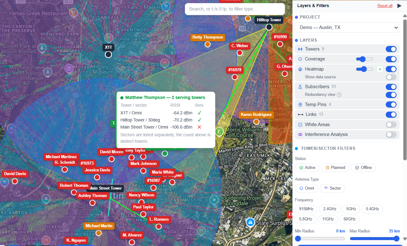
- Green — 2+ towers: more than one tower can serve this subscriber. Losing any one of them still leaves a working option.
- Amber — 1 tower only: genuinely served right now, but with no backup. This is the bucket worth acting on.
- Red — no tower: no tower can serve this subscriber to your project's standard. These are the same subscribers the normal view shows as unserved.
- Grey — not computed: this project hasn't been through a coverage recalculation since this view became available, so there's no redundancy data for it yet. See below.
The filter chips below the toggle switch to match, so you can isolate just the amber "one tower only" subscribers and work through them. Hovering any marker shows a table of every tower/sector that reaches it, its predicted signal, and a ✓ or ✕ for whether that option is actually strong enough to count.
What counts as a serving tower
A tower only counts toward redundancy when it could genuinely serve the subscriber on its own — being in range isn't enough. Each candidate's own predicted signal is checked against the same thresholds the rest of your project uses, so an option that's technically in range but too weak to sell is listed in the hover table with a ✕ and does not count. This is why a subscriber can show several rows in the table but still be amber or red.
If two sectors on the same tower both reach a subscriber, that's still one tower — losing that tower loses both. The hover table lists sectors separately (useful detail), but the color and count are always per distinct tower. Where that difference applies, the table says so explicitly, so it never looks like it disagrees with the marker.
"No serving tower" and "unserved" mean the same thing — a subscriber shown red here is red in the normal view too. The two views are built so they can't disagree about the same marker. Note that redundancy counts real options, independent of which tower is currently assigned: a subscriber whose assigned tower is marginal can still be green if a different, genuinely strong tower also reaches them.
First use: one coverage recalculation
The alternate towers each subscriber could use are worked out during coverage classification, but they weren't stored before this view existed — so an existing project shows every marker grey the first time you open it, with a prompt offering to Recalculate coverage. Running it once fills in the data for the whole project; after that it stays current automatically, updated whenever coverage is reclassified (adding, editing, moving or deleting a tower or sector, or editing a subscriber).
That recalculation is never started automatically — switching a view should not kick off a project-wide recompute without you asking. It uses exactly the same signal checks a normal reclassification already runs, so expect it to take about as long as one for a project of your size.
Redundancy depends on the per-candidate signal check, so it needs RSSI classification or throughput qualification switched on in Project Settings. On a project using purely geometric coverage, this view will tell you so and no recalculation will help until one of those is enabled — because without them the per-tower signal numbers it counts are never computed at all.
No extra computation
This view adds no new terrain, LiDAR or propagation work. Coverage classification already tests every tower/sector that could reach each subscriber, at full precision, and then keeps only the best one — the alternates were already being calculated and thrown away. This view simply keeps them. It is Pro plan (and trial) only; on other plans the toggle is visible but disabled, so you can see it exists without being able to switch to it.
Subscriber Statistics
Subscriber statistics are visible in multiple places:
- Map stats bar (bottom-left) — live counts for the currently loaded data
- Project view dashboard — served/unserved/potential/unknown with coverage percentage
- Subscriber list — filterable by status, searchable by name and address
Coverage % = served ÷ (served + unserved + unknown) × 100. Potential subscribers are excluded from the denominator since they are not confirmed customers.
Team Management
Projects can be shared with other GridVisio users as collaborators. Each collaborator has a role that determines their level of access.
Project view → Team buttonRoles
- Owner — full access, can invite and remove team members, can delete the project
- Editor — can add/edit/delete towers, subscribers, pins, and links. Can configure project settings
- Viewer — read-only access to the project and map. Cannot make any changes
Inviting a collaborator
- 1Go to Team page
From the project view, click the Team button in the header.
- 2Enter email and role
Type the invitee's email address and select their role (Editor or Viewer).
- 3Send invitation
The invitee receives an email with an accept link. Until they accept, their status shows as "Pending".
Free plan: no collaboration. Trial/Starter: 3 collaborator seats per project. Pro: 10 seats per project.
Shared Maps
Shared maps are read-only, publicly accessible links to a project's map view. No GridVisio account is required to view a shared map.
Project view → Shared Maps Map → Export ▾ → Share Map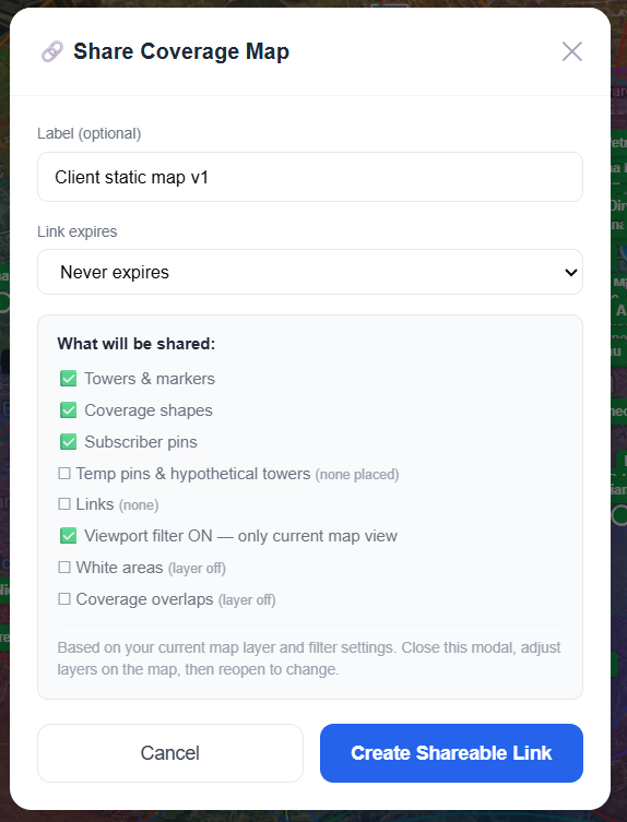
Creating a shared link
- Label — optional name for the link (e.g. "For client review")
- Expiry — never, 7 days, 30 days, or 90 days
- Content — choose what to show: towers, coverage, subscribers, heatmap
- Viewport — when sharing from the map, optionally lock the shared view to the current viewport bounds
The Heatmap option shows the single-color "covered / not covered" view of any already-generated RF Propagation Heatmap data for the project — not the internal multi-color signal-strength bands, which stay map-only. It defaults off (unlike the other three, which default on), since a project can easily have no generated heatmap yet when a link is created. When sharing directly from the map, this mirrors whatever the map's own Heatmap layer toggle is currently set to, the same way the other three options already do.
Managing links
From the Shared Maps page you can activate/deactivate links (without deleting them), see access counts and last viewed date, and delete links permanently.
Free plan: no shared links. Trial: 3 links. Starter: 10 links. Pro: unlimited.
Export Options
GridVisio supports multiple export formats for different use cases.
Map → Export ▾ menu Sidebar → Network → ExportsXLSX, PDF, PNG, KMZ, and Shapefile exports require a Starter or Pro plan. CSV export is available on all plans. LoS PDF and PNG exports are available on all plans.
PNG map export
Exports the current map view as a high-resolution PNG image. Includes all visible layers at the current zoom level.
PDF export
Generates a formatted PDF report with the map image, project summary, and tower/subscriber statistics.
XLSX export
Exports tower and subscriber data as a structured Excel spreadsheet with multiple sheets. The sector radius and tower height columns are named and valued in your own Distance Unit preference (radius_km/height_m or radius_mi/height_ft) — check the header before feeding the file into another tool.
CSV export
Simple comma-separated export of subscriber or tower data. Available on all plans.
KMZ export
Exports towers (points), coverage sectors (polygons, colour-coded), subscribers (colour-coded by status), the RF Propagation Heatmap (as a georeferenced image overlay, if the project has one generated — Pro/trial only), and saved LoS Checker links (as coloured lines) as a KMZ file. Opens in Google Earth and GIS tools such as QGIS. Towers/sectors/subscribers/heatmap respect the active viewport filter; saved links always export for the whole project.
Shapefile export
Exports a .zip containing three Shapefile layers: towers (points), coverage sectors (polygons, same shape as the KMZ export), and subscribers (points, with a status attribute). A single Shapefile can only hold one geometry type, which is why this is a small bundle of three complete file-sets rather than one file — standard practice for a multi-layer Shapefile export. Opens in QGIS, ArcGIS, and any other Shapefile-reading GIS tool. The heatmap layer isn't included (a Shapefile can't represent raster data), and saved LoS Checker links aren't included in this export. Towers/sectors/subscribers respect the active viewport filter.
LoS PDF / PNG
Single-page PDF or PNG of the LoS Link Check terrain profile with Fresnel zone, LoS status, and path loss. Available on all plans.
BDC & BEAD Export
GridVisio supports export in the formats required for US government broadband funding programs.
Map → Export ▾ → BDC Export / BEAD ExportBDC and BEAD exports require a Starter or Pro plan.
BDC (Broadband Data Collection)
The FCC's Broadband Data Collection program requires ISPs to submit coverage data in a specific format. GridVisio's BDC export generates a file conforming to the BDC specification, including coverage polygons and technology codes derived from your sector frequency bands.
BEAD (Broadband Equity, Access, and Deployment)
The BEAD program requires ISPs to identify unserved and underserved locations for federal grant applications. Clicking BEAD Export opens a modal where you fill in applicant and project details, then start the export — terrain/signal verification for every location in scope runs automatically as part of it, no separate step required.
What the export produces
The BEAD export downloads as a ZIP archive containing four files:
Executive Summary PDF
Formatted report with applicant details, network summary (active towers, sectors, coverage radii, frequency bands), unserved location cluster map, tower table, FCC classification summary (see below), and a BEAD readiness checklist.
Location Inventory CSV
Every subscriber in the export area: name, address, coordinates, BEAD status, cluster assignment, and LoS status (always present). Plan-qualifying exports (Pro/Trial) additionally get predicted RSSI, serving tower/sector, predicted throughput, and an FCC downlink classification column — see below.
White Areas GeoJSON
Cluster polygons as a GeoJSON FeatureCollection, ready to load in QGIS, ArcGIS, or any GIS tool that accepts GeoJSON.
README.txt
Plain-text description of each file and guidance on how to use the package in a BEAD application.
BEAD export modal
The modal has two sections: applicant information and project details. All fields are saved automatically in your browser (localStorage) so they are pre-filled the next time you open the modal — even for a different project. Applicant-level fields (name, EIN, address, contact, email, phone, state) are shared across all projects; project-specific fields (project description, target area, tech type, etc.) are saved per project.
Automatic verification (queued export)
Building a BEAD export runs in the background rather than blocking your browser on one long request. After you click Download BEAD Bundle:
- A small progress banner ("Building BEAD export…") appears at the top of the map. You can keep working — it polls for status every few seconds.
- The export first ensures every subscriber in the export area has a real, stored signal measurement (predicted RSSI, LoS/Fresnel verdict, and — if a CPE model resolves — predicted throughput). A subscriber that was already measured (from a prior recalculation, or a prior export) is not re-measured — only ones genuinely missing a measurement are computed, which is why a repeat export on the same project is typically much faster than the first one. Once at least one location needs measuring, the banner also shows a running count ("N of M subscribers measured").
- This is the exact same 50-sample, LiDAR-aware engine used everywhere else in GridVisio (the map's own RSSI verification, the RF Heatmap) — not a separate, faster, less-precise bulk check. Every active sector that geometrically reaches the location is tested (same multi-candidate matching described under Classification), and the best-performing one is used, so the export's serving tower/sector can legitimately differ from the one shown elsewhere if the project's classification settings were changed since the last recalculation. This measurement pass always runs regardless of whether the project has RSSI/throughput verification turned on at all — it can only fill in a number, never change a subscriber's served/unserved status. There is no manual "Verify with LoS" step or subscriber cap to configure; every location in the export's scope gets a result.
- Once every location is measured, the PDF/CSV/GeoJSON are built directly from those stored values and the ZIP downloads automatically.

Every export gets the LoS Status column (Reachable / Terrain-blocked / Beyond distance cap / Not verified) regardless of plan. Predicted RSSI, serving tower/sector, predicted throughput, and the FCC classification column additionally require the project owner's plan to include RSSI/throughput prediction (Pro or Trial) — on a Starter-plan project those columns are simply omitted from the CSV rather than shown blank. The underlying measurement is still stored either way (so it's ready immediately if the plan is upgraded later); only which columns the export shows depends on plan.
A separate bucketing from your project's own BEAD Status column, computed directly from stored predicted downlink throughput against the FCC's own 25 / 100 Mbps lines (Unserved <25, Underserved 25–100, Served ≥100). FCC BEAD classification shown here is based on DOWNLINK throughput only — the FCC's official definitions use a two-sided threshold (25/3 Mbps for unserved, 100/20 Mbps for underserved), and GridVisio has no uplink propagation model, so treat this bucket as a downlink-only planning approximation, not an official BEAD determination. Verify uplink capability separately before submission. Only appears when predicted throughput is available (Pro/Trial plan, a resolvable CPE model).
Export Area: Full Project vs. Polygon
Clicking BEAD Grant Package opens a small Export Area panel before the main modal, letting you choose what the export covers:
- Full Project (default) — every subscriber location in the project is included; the PDF's tower table shows up to 15 rows.
- Polygon — click points on the map to draw a custom area, then click Finish to close the shape. Only subscriber locations inside the drawn polygon are included in the CSV, the unserved-cluster detection (and its GeoJSON), and the PDF's tower table (capped at 10 rows). A live location count updates once the shape is closed. Drag any vertex to reshape it afterward, or use Draw new / Remove to start over or clear it.
The drawn polygon is resolved on the server against your project's full data every time it's used — it does not depend on what the map happens to have loaded or rendered at the time, and it's remembered per project (saved in your browser) so it's still there the next time you open the panel. Click Next step to continue to the applicant/project details modal, or Edit from inside that modal to come back and change the area. In both scope modes, an overflow note in the PDF lists how many additional towers exist and includes project-wide network totals.
PDF structure
- Section 1 — Current Network Summary — five coloured stat cards (active towers, sectors, average radius, max radius, frequency bands) on a single row, followed by the BEAD eligibility table, an FCC downlink classification table (Pro/Trial plans with throughput data — see above), a tower table, and an unserved location cluster table
- Section 2 — Applicant Information — organisation name, EIN, address, state, primary contact
- Section 3 — Project Description — free-text description with newlines preserved
- Section 4 — BEAD Readiness Checklist — checklist of required documents referencing the companion CSV and GeoJSON files
- Section 5 — Additional Resources
Unserved location clusters in the PDF and GeoJSON are detected using the same DBSCAN algorithm as the White Area Detection map layer. The algorithm groups unserved/unknown subscribers within the configured epsilon radius and minimum point threshold, computes a convex hull around each cluster, and buffers the polygon outward for visual clarity. Cluster parameters are taken from Project Settings → White Area Detection.
Coverage Widget
The Coverage Widget embeds a compact interactive checker on your website. Visitors enter their address or drop a pin on the map, and the widget tells them whether they're in your service area — no GridVisio account required. With lead capture enabled it also collects visitor contact details and runs a full line-of-sight analysis, sending you a notification with the result.
Project view → Coverage Widget buttonThe Coverage Widget is a Starter plan feature and above (also available during the 14-day trial). Starter widgets test up to 3 nearby towers per lead; Pro widgets test up to 6.
Widget modes
Each widget has one of three modes, set in the widget settings:
Coverage only
Address → map → Check. Shows covered / not covered. No contact details collected. Lightest option.
Coverage → Lead
Check coverage first. If covered (or always, if configured), the contact form appears. Captures qualified leads.
Lead form first
Contact form appears first. After filling it, the visitor picks their location and checks coverage. Captures every visitor, even unserved ones — useful for building a waitlist.
Visitor flow — Coverage only
- Enter an address or drop the pin on the map.
- Click Check — the server runs the same line-of-sight analysis described below (see What the LoS analysis covers) and returns a result.
- Result: Covered (with serving tower), ~ Marginal, or Not covered. No contact details are collected in this mode, so nothing is ever saved as a lead.
Visitor flow — Coverage → Lead
- Enter address / drop pin → Click Check. Result shows instantly.
- If covered (or unserved capture is enabled): the location picker collapses and the contact form appears below the result.
- Visitor fills in name / email / phone → Click Send. Full LoS analysis runs server-side.
- Fields become read-only, a thank-you message appears, and a ← New inquiry button resets the widget for the next visitor.
Visitor flow — Lead form first
- Contact form is shown immediately — name / email / phone → Click Next →.
- Location picker appears (address, map, GPS). Visitor picks location → Click Check.
- Full LoS analysis runs. Coverage result + thank-you shown. ← New inquiry resets to the contact form.
Every check the widget performs — in all three modes, whether or not a lead ends up being captured — runs the same real line-of-sight analysis against your nearest towers (configurable, up to 3 on Starter / trial, up to 6 on Pro). For each nearby tower, GridVisio first checks whether any of that tower's active sectors actually covers the direction toward the visitor (the same geometric test used elsewhere — see LoS Link Check's Ant. height A / B note). It fetches terrain elevation in parallel, adds estimated clutter height (vegetation/buildings, the same NLCD/WorldCover data used by the map's LoS Link Check tool) on top of bare elevation, checks Fresnel zone clearance against that clutter-raised profile using the same 60% rule as the map tool, and computes free-space path loss for each tower using that sector's real antenna height and frequency band. If a tower has more than one active sector, the frequency used is taken from the first one found, defaulting to 5.8 GHz if none have a usable frequency band set — see sector Status. When a lead is captured, results are stored with it and included in the email notification; every check's per-tower results are also returned directly in the API response — see Public API.
The LoS analysis above always runs on bare elevation + estimated land-cover height, the same engine used everywhere else in GridVisio. The Enable LiDAR widget setting additionally pulls real USGS 3DEP LiDAR measurements (where the free public dataset has coverage — see 3DEP LiDAR) into that same analysis for higher precision. It's off by default because a live LiDAR fetch takes noticeably longer to respond than clutter alone — turn it on if check accuracy matters more to you than response speed. With it on, the first check in an area can take up to about 40 seconds while the real measurements for each nearby tower's path are fetched; later checks of the same paths are answered from the saved result in a second or two.
If none of a candidate tower's active sectors geometrically cover the visitor's direction — or the tower has no active sectors at all — that tower is left out of the analysis entirely rather than falling back to a generic height and risking a misleading "served" result for a direction your actual antennas don't point toward. A Planned or Offline sector pointing exactly at the visitor does not save the tower from exclusion — by design, since a real visitor should never be told they're covered by infrastructure that isn't live yet. The lead's tower table (in both the Lead Inbox and the notification email) still lists the tower, marked "Excluded — no sector covers this direction", so you can see why a geographically close tower didn't come up as a real candidate. This is different from the map's LoS Link Check tool and the BEAD bulk verification, both of which fall back to the tower's structure height instead of excluding it, since those are operator-initiated exploratory checks rather than a public-facing "are you covered" answer.
Widget settings
- Mode — Coverage only / Coverage → Lead / Lead form first
- Enable LiDAR — applies to every mode; pulls real LiDAR measurements into the LoS analysis for higher precision, at the cost of a slower response. Off by default — see Enable LiDAR above.
- Allowed Domains — comma-separated list of domains allowed to embed the widget's iframe. Required for the embedded widget to complete real checks — leave it blank and the iframe still loads, but anonymous visitors' checks are rejected until a domain is set. See Public API for exactly what this does and doesn't protect against.
- API Secret — Bearer credential for calling the Coverage Check API directly from your own server, bypassing the iframe. Generate/regenerate it next to the webhook secret. See Public API for the exact header format.
- Form fields — choose which fields (name, email, phone) to show and which are required
- Towers to test — up to 3 (Starter / trial) or 6 (Pro) towers used for the LoS analysis on lead submission
- Capture when unserved — in Coverage → Lead mode, also show the form when the visitor is outside coverage
- Brand colour — hex colour applied to the Check / Send buttons and focus rings
- Thank-you message — custom message shown after a successful lead submission
- Redirect URL — instead of a thank-you message, redirect the visitor to a page on your site
- Notification email — address that receives the lead notification email
- Webhook URL + secret — optional POST to your CRM or automation tool, signed with HMAC-SHA256
Embedding the widget
- Open the project → click Coverage Widget in the header.
- Click Enable Coverage Widget and configure the mode and settings.
- Set Allowed Domains to the domain(s) you'll embed on — required, see below.
- Copy the generated
<iframe>snippet and paste it into your website HTML.
The embed code uses height="330", which fits all three widget modes and their post-submission states. Do not reduce this value.
The iframe will render even without an Allowed Domain configured — but real visitors won't be able to complete a check until you set at least one. This is deliberate: it's what actually stops a copy of your embed code (or just your widget's URL, visible in any page's source) from being used to run coverage checks from somewhere else entirely. See Public API for exactly how this is enforced.
Managing leads
Captured leads appear under Leads in the sidebar. Each lead shows the visitor's contact details, the address they checked, the coverage result, and a per-tower LoS breakdown. You can:
- Update the lead status (New → Contacted → Qualified → Converted / Lost)
- Add internal notes
- Filter by date, classification, or tower
- Export all leads to CSV in bulk
An unread badge on the Leads sidebar entry shows how many new leads haven't been opened yet.
Token management
- Regenerate token — issues a new embed URL and invalidates the old one. Update your website after regenerating.
- Regenerate API secret — invalidates the current one immediately; update it in any server-side integration calling the Coverage Check API directly. Doesn't affect the embedded iframe at all, which doesn't use this secret.
- Disable widget — deactivates immediately; visitors see a "temporarily unavailable" message.
Public API
Everything the embedded widget's own JavaScript does, you can also do yourself: call the same endpoint directly from your own server or front end instead of embedding the iframe. This page documents the first endpoint made available this way — the Coverage Widget's check call. More endpoints will be added here over time as GridVisio exposes further functionality for direct integration.
The embedded iframe is tuned for speed — a real visitor is waiting on your page, so it uses a fixed-resolution engine (the same one that also powers the instant coverage-map check). A call authenticated with your API secret instead runs the same per-link precision engine used everywhere else in GridVisio (LoS Link Check, POP Scan, subscriber classification) — testing each candidate tower individually against a 2 m-resolution terrain grid (30 m where LiDAR coverage doesn't reach) instead of a shared, fixed 50-sample profile. It's slower — expect it to take noticeably longer, especially the first time a given area is checked — but the result is the same accuracy every other tool in the app relies on, which matters if you're feeding it into your own downstream decisions. Your widget's Enable LiDAR setting still applies either way: if you've turned it off, a direct API call still skips the extra LiDAR fetch entirely rather than silently overriding your choice.
The widget token in the URL is not sufficient on its own to call this endpoint — it identifies which project to check, but every call must additionally prove it's coming from one of two legitimate places:
- The embedded iframe (a real visitor using the widget on your site) — handled automatically, nothing to configure beyond Allowed Domains (see below).
- A direct/server-to-server call like the one this page documents — authenticate with your widget's API secret (Coverage Widget settings page, next to the webhook secret), sent as a header, never in the URL:
A request with neither a valid embedded-widget session nor a valid API secret gets a 401.
Coverage Check
POST/api/widget/{token}/check
Same domain as your widget's embed URL (shown on the Coverage Widget settings page) — for example:
Request body
| Field | Type | Required | Notes |
|---|---|---|---|
lat | float | Yes | Latitude of the address to check, −90 to 90. |
lng | float | Yes | Longitude of the address to check, −180 to 180. |
website | string | No | Honeypot — leave empty. A non-empty value is silently treated as a bot: you get a normal-looking "not covered" response back, with no LoS work done and nothing saved. |
source_url | string (URL) | No | Must be a fully-qualified URL if you send it (e.g. https://example.com/page) — a non-empty value that isn't a valid URL returns a 422. Stored as-is on any captured lead; purely informational, not used for anything else. |
name, email, phone, address | string | Depends on mode | Lead-capture fields. Ignored in Coverage only mode. In Lead form first mode, email or phone is required. In Coverage → Lead mode, send lat/lng alone first for the instant result, then re-POST with whichever of these you collected — the server enforces the same Required checkboxes configured under Widget settings → Form fields on that second call. |
Response body
| Field | Type | Meaning |
|---|---|---|
covered | bool | Whether the location is served — true only when the LoS analysis reaches the "serviceable" tier, not just geometrically inside a sector's radius/beamwidth. |
served_by | string / null | Name of the serving tower. |
serviceable | bool | Same value as covered — kept alongside it for a clearer field name. |
classification | string | "serviceable", "marginal", or "no_service". |
best_tower | string / null | Same value as served_by. |
message | string | Human-readable result, suitable to show directly to a visitor. |
tower_results | array | One entry per candidate tower analysed — see below. The same detail saved on a captured lead, always included here whether or not a lead ends up being saved. |
redirect_url | string / null | Configured redirect URL, if any (Coverage → Lead / Lead form first modes). |
lead_captured | bool | true only when this call actually saved a lead (contact fields present, per mode's rules). |
Each tower_results entry
tower_id,tower_name,distance_kmin_sector(bool) — whether an active sector was found covering the visitor's direction from this tower.excluded+exclusion_reason— present instead of the fields below whenin_sectoris false (see A nearby tower can still be excluded above).served(bool),tier("clear"/"borderline"/"obstructed", or"unavailable"when the terrain elevation for that path could not be fetched — no verdict is given,clearance_pctisnull,elevation_unavailableistrue, and the overallclassificationis"marginal"rather than a false "no service"),clearance_pct(Fresnel-zone clearance),fspl_db(free-space path loss)terrain_source("bare"/"clutter"/"lidar"),lidar_coverage_pct,lidar_provider— which elevation data actually backed the worst point on this tower's path;lidar_coverage_pctis 0 unless Enable LiDAR (see Widget settings) is on for this widget.sector_name,rssi_dbm,throughput_mbps,modulation— only present when the project owner's plan includes predicted RSSI/throughput (Pro).
Example response
Error response — not authenticated
HTTP 401. Also returned for a stale or expired embedded-widget session — this is stateless and short-lived, so a visitor who keeps the same tab open for a long time may need to reload before their next check.
Error response — invalid source_url
The Coverage Check endpoint allows 30 requests per minute. That limit is tracked by the calling IP address, not by widget token — if you call this endpoint from your own server rather than embedding the iframe (where each visitor's own browser calls it from their own IP), every request your server makes shares one 30-per-minute allowance, no matter how many different widgets or visitors it's calling on behalf of. Exceeding it returns an HTTP 429 Too Many Requests response. The widget's iframe page itself (GET /widget/{token}) has no separate rate limit.
Allowed Domains is checked once, when the iframe itself loads (GET /widget/{token}) — that's the one request in this whole flow whose Referer genuinely names the page embedding it, since a browser can't be made to lie about that. A verified match there mints a short-lived session the iframe's own checks use automatically; you don't do anything for this path beyond configuring the domain(s). It has no effect on direct calls like the one this page documents — a server-to-server integration doesn't carry a page Referer, so there's nothing to check. That's what the API secret is for instead: authenticate directly with it, independent of any domain. Configure whichever one(s) match how you're integrating; a widget can support both an embedded iframe on an allowed domain and a separate server-side integration with the secret at the same time.
Project Settings
Project settings configure per-project defaults and algorithm parameters. Settings apply to all users working on the project. The page is organized into tabs — Tower Marker, Sector Defaults, Frequencies, Equipment Presets, RF Heatmap, Classification, Clutter, Clustering, and White Area Detection — with one Save Settings button that saves whichever tab is active plus any others you've changed; it isn't per-tab. Changing a field that affects stored subscriber classification (see Classification below) shows a confirmation step naming how many subscribers will be re-classified before Save actually runs — recalculation itself then follows with a real progress bar, the same one the map's own Recalculate Coverage button uses.
Project view → Settings button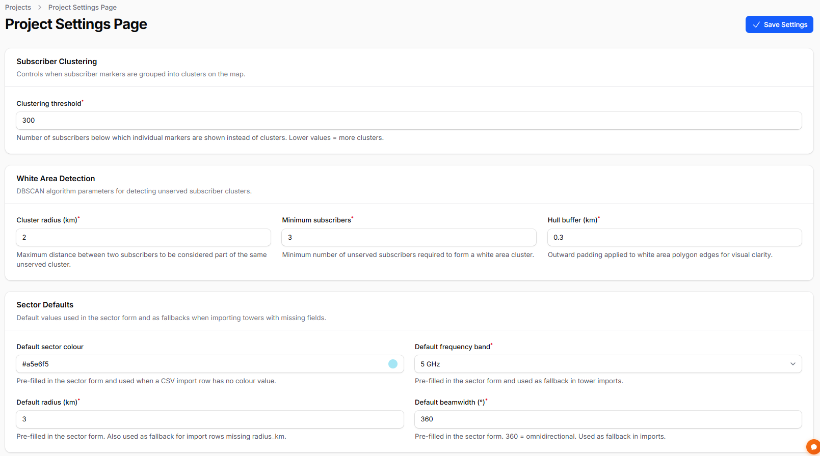
Subscriber clustering
- Clustering threshold — subscriber count below which individual markers are shown instead of clusters. Default: 150. Lower = more clusters at higher subscriber counts.
White area detection
- Cluster radius — DBSCAN epsilon parameter. Default: 2.0 km
- Minimum subscribers — DBSCAN min_points parameter. Default: 3
- Hull buffer — convex hull outward padding. Default: 0.3 km
Sector defaults
These values pre-fill the sector form when adding a new tower, and serve as fallbacks when importing towers with missing sector fields.
- Default sector colour
- Default frequency band
- Default radius
- Default beamwidth (°)
Frequencies
This project's own list of assignable frequency bands — every sector-editing screen (map and admin) only offers values from this list, shown as a compact grid of one field per frequency. A new project starts with a default set of 19 common bands (900MHz through 80GHz, plus common LTE/LoRa numeric bands); add your own precise value if what you need isn't there, or delete ones you don't use. A frequency still used by an enabled equipment preset for this project can't be removed until that preset is disabled first, in the Equipment Presets tab below.
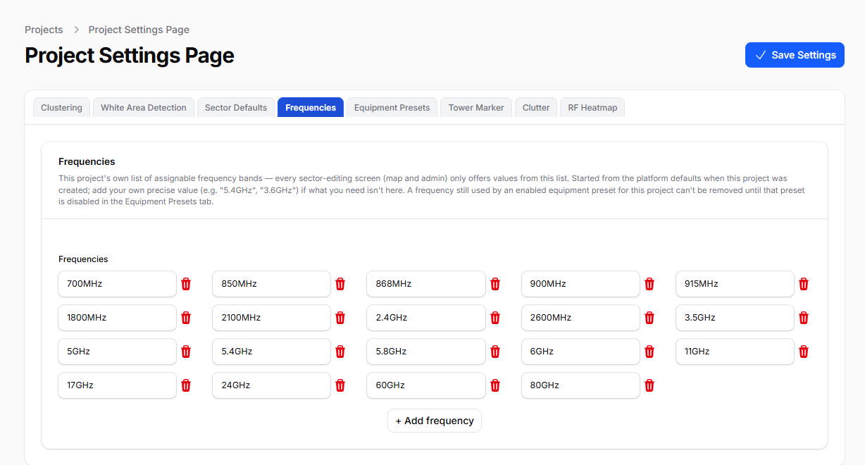
Equipment Presets
Which of your account-level equipment presets are offered when filling a sector's RF fields on this project's map and tower forms. New projects start with every existing preset enabled; manage the presets themselves (create, edit, delete) from the Equipment Presets page under Network in the sidebar. Enabling a preset here automatically ensures its frequency is on this project's Frequencies list above.
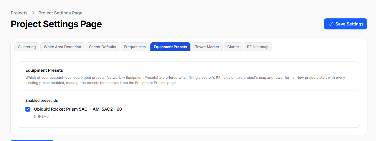
Classification
Turns on real signal-strength verification for subscriber coverage status, on top of the geometric sector-membership test described under Subscribers above.
Verify with predicted RSSI is enabled when a project is created, so subscribers show a predicted signal (and a predicted throughput, where a CPE model resolves) without you having to find a setting first. Existing projects are unchanged — whatever they were set to, they stay set to. Turning it off returns a project to purely geometric served/unserved. Note this does more than add numbers: a geometrically-served subscriber with a weak predicted signal becomes Marginal or Unserved, so a project with it on will show statuses a purely geometric one would not. It also means coverage recalculation does real terrain and propagation work, which takes meaningfully longer than a geometric-only pass on a large import.
- Verify with predicted RSSI — runs a real signal prediction, using this project's configured propagation model(s) (the same engine as the RF Heatmap and LoS Link Check), for every subscriber, not just a geometric check. A geometrically-served subscriber whose predicted signal falls below Minimum usable signal (dBm) becomes Marginal; below Hard floor / receiver sensitivity (dBm) it downgrades further to Unserved. A missing prediction (terrain data unavailable, etc.) never downgrades anyone — the geometric result stands.
- Allow RSSI to extend beyond configured radius — only meaningful with the toggle above on. Treats a sector's radius as a planning boundary rather than a hard coverage edge: a subscriber just outside the radius but still inside the beam can be promoted to Served if its predicted signal clears the threshold. Off by default — leave it off if your radii represent real business limits (install crew reach, franchise boundaries), not just "how far the antenna throws power."
- Extend margin (%) — only shown when the toggle above is on. A slider from 5% to 30% (default 15%) that sets how far beyond a sector's own radius a subscriber can still be considered: each sector's own search reach is
radius_km × (1 + margin% / 100)— a 10 km sector at the default 15% margin reaches 11.5 km, a 20 km sector reaches 23 km. On Free, Trial, and Starter plans this per-sector reach is additionally capped at your plan's flat maximum RF link distance (5 km Free/Trial, 10 km Starter); on Pro (and for admin accounts) there is no additional cap beyond the formula itself — adjust either the sector's own radius or this margin to reach further. Whenever a tower or sector edit could change who qualifies, the map shows the margin percentage (and plan cap, if any) being used before recalculating so the effect is never a surprise. - Require minimum throughput + Minimum throughput (Mbps) — an independent, further gate: a subscriber whose predicted throughput (from its CPE model's real MCS/sensitivity table — see Equipment Presets) falls below this number downgrades to Unserved, regardless of signal strength. Needs a resolvable CPE model (the subscriber's own, or this project's Default CPE model above) — without one, throughput stays honestly blank and never downgrades anyone.
Predicted RSSI/throughput numbers are computed and stored whenever either toggle is on, and are also computed on demand for a BEAD export regardless of these toggles — see BDC & BEAD Export. Viewing the stored numbers (the map popover, the subscriber list) requires a Pro or Trial plan; the toggles and thresholds themselves are configurable on any plan, but only take effect once the project owner's plan qualifies.
When either toggle above is on, verification doesn't just re-check the single tower/sector the geometric test happened to pick — it tests every active sector, on every tower, whose radius and beam genuinely reach the subscriber (including any sector that only qualifies through the extend-beyond-radius margin, if that's on), using the exact same terrain/LiDAR engine a manual LoS Link Check uses for one link — never a coarser or faster bulk approximation. Whichever candidate actually performs best is kept: highest predicted RSSI when RSSI verification is on (RSSI is the ranking signal even when throughput qualification is also on — throughput is always a secondary gate applied after, never the tiebreaker), or highest predicted throughput when only the throughput checkbox is on. A subscriber can therefore end up served by a genuinely different tower/sector than the one the plain geometric test would have picked, whenever a farther or differently-angled sector turns out to have a clearer path or stronger real-world signal.
The geometric served/unserved test (see Subscribers) checks every sector regardless of status — a subscriber can show as geometrically "Served" by a Planned or Offline sector, since this is a planning tool and a not-yet-built sector's footprint is still useful to see. Verification's search for a better candidate (a farther or differently-angled tower that might outperform the geometric pick) only ever considers active sectors — but a subscriber's own already-resolved serving sector is always tested too, regardless of its status, so a subscriber served by a Planned or Offline sector still gets a real, honest signal reading against that specific sector. It just can't be outranked by an inactive alternative elsewhere. See sector Status for how every other tool in GridVisio treats sector status.
Throughput prediction needs a real CPE hardware model to read modulation/sensitivity numbers from (the subscriber's own CPE model, or this project's Default CPE model — see Equipment Presets). A candidate tower/sector is only ever paired with that CPE model for a throughput prediction when their frequency bands actually match — a CPE can't meaningfully predict throughput on a frequency it doesn't operate on. A frequency mismatch never removes that candidate from consideration, though: it's still fully tested for RSSI and can still win the ranking on signal strength alone — it simply never gets a throughput (Mbps) number, the same honest "no compatible hardware to predict from" result you'd see for any subscriber with no CPE resolved at all.
When that happens, the subscriber's map tooltip and Edit modal can still show a Mbps figure alongside a small orange ≈ badge — hover it for the explanation. That number is an estimate, computed from the resolved CPE's own modulation curve evaluated against the real, already-computed RSSI for that link; it's informational only and never factors into serving-tower selection, ranking, or served/unserved status, all of which still run on the frequency-matched result above. It's a "what a compatible radio would likely deliver at this signal level" figure, not a claim about the exact hardware that would be installed.
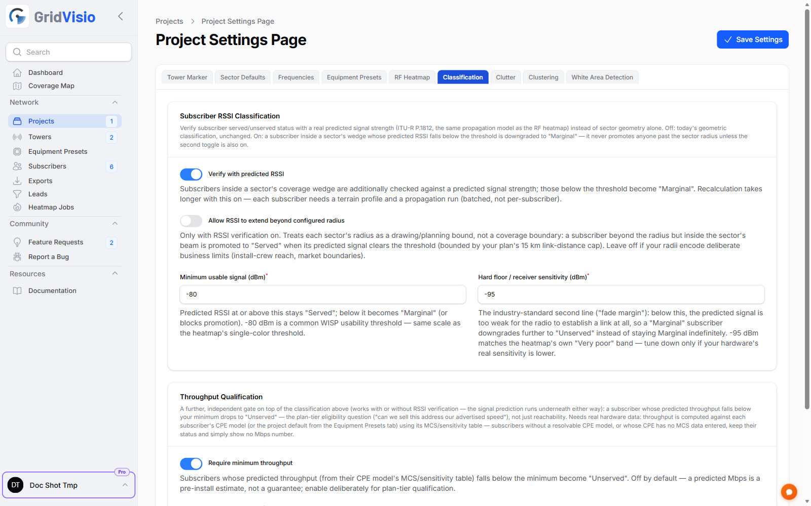
Tower marker
- Marker fill colour — colour of the tower dot on the map and its label background
- Marker border colour — stroke colour around the tower dot
RF Heatmap
Both the link-budget assumptions and the display/colour settings live together in this one tab. See RF Propagation Heatmap for what these control — both display modes render from the same computed data, only the threshold/colours applied here differ. The multi-color signal-strength bands are shown as a compact table, one row per band.
- Assumed CPE antenna gain (dBi) — a project-wide stand-in for "a typical subscriber radio," since there's no real subscriber to read a value from for a hypothetical heatmap grid cell. Default: 20 dBi (up to 50 dBi accepted, for projects modeling 60 GHz mmWave CPE).
- Assumed cable/connector loss (dB) — same reasoning, typical short jumper + connector loss. Default: 1.0 dB.
- Overlay opacity — how solid the public/embeddable single-color view looks. From 10% to 100%, default 50%. Display-only — changing it re-colours the already-computed heatmap the next time it's rendered, it never clears or recomputes any heatmap. The internal map's own Heatmap layer has a separate, session-only live opacity slider instead (in the Layers panel, next to the layer toggle) — this project setting only seeds that slider's starting position, it doesn't otherwise control the internal map.
- Minimum usable signal (dBm) — the single threshold for the public/embeddable single-color view: points at or above this show as "covered". Default: −80 dBm.
- Covered colour — the single-color view's "covered" colour.
- Multi-color signal-strength bands — a list of dBm ranges and colours for the internal map layer, ordered strongest to weakest. Either end of a band can be left blank for an open-ended range (the strongest band has no upper limit, the weakest has no lower limit).
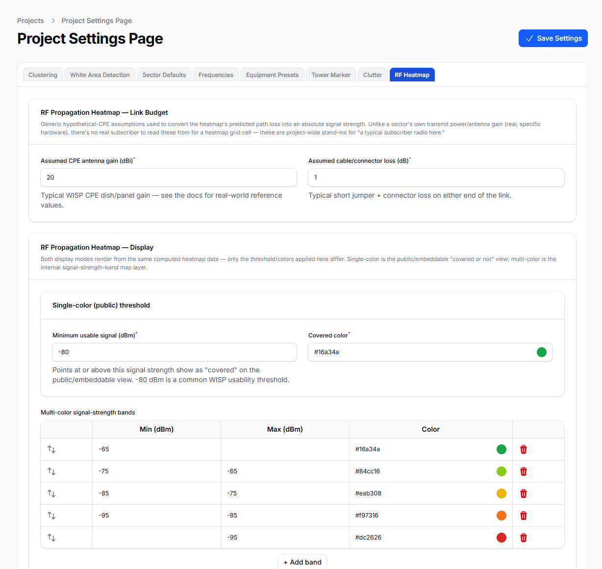
Account Settings
Account settings manage your personal profile and subscription.
Sidebar user menu (bottom-left avatar) → Account Sidebar user menu (bottom-left avatar) → Billing & PlanAccount page
- Update your name and email address
- Choose your preferred currency (USD or EUR) and distance unit (kilometers or miles)
- Change your password
- Delete your account (see below)
Your Distance Unit preference (Account page, next to Preferred Currency) controls how every radius/distance AND every height/elevation value is displayed and entered throughout GridVisio — the map, tower/sector/subscriber forms, CSV import/export, PDF/XLSX/KMZ exports, and the lead-notification email. Choosing Miles switches heights to feet too (tower structure height, antenna/CPE mounting height, terrain elevation) — matching how the US tower industry actually states height, in feet, never meters. It's purely a display setting: every number in this documentation is stated in kilometers/meters, and GridVisio's internal calculations always use kilometers/meters regardless of your preference, so switching units never changes a computed result, only how the numbers are shown to you. New accounts are asked to choose on first use (a prompt appears on the Dashboard right after login, and again on the map if skipped); change it any time on the Account page.
Deleting your account
Account deletion is available in the Danger Zone section at the bottom of the Account page. Deletion is not immediate — the following process applies:
- Click Delete Account and confirm your email address
- A confirmation email is sent with a cancellation link
- A 7-day grace period begins — your account remains fully accessible during this time
- To cancel the deletion, click the link in the email or click Cancel Account Deletion on the Account page
- After 7 days, your account and all data are permanently and irreversibly deleted: projects, towers, sectors, subscribers, coverage data, drive tests, LoS links, shared maps, and exports
All data is permanently deleted at the end of the grace period with no recovery option. Use the export tools (CSV, XLSX, PDF, KMZ) to save any data you need before requesting deletion.
Billing page
- View current plan and trial status
- See usage vs limits for projects, towers, subscribers, and saved links
- Upgrade, downgrade, or cancel your subscription
- Switch between monthly and annual billing
- Switch between USD and EUR currency
- Access the Stripe customer portal to manage payment methods and invoices
Feature Requests
Suggest new features and vote on proposals from other users. The roadmap is shaped by the community.
Sidebar → Community → Feature RequestsSubmitting a request
Any registered user can submit a feature request with a title and description. Requests are reviewed by the GridVisio team before being published for voting.
Voting
Once approved, feature requests are open for voting. Vote weights depend on your plan:
- Free / Trial: 1 vote weight
- Starter: 2 vote weight
- Pro: 3 vote weight
Each user can vote once per feature request. Implemented features are marked accordingly.
Bug Reports
Report issues or unexpected behaviour directly from within the app.
Sidebar → Community → Report a BugSubmitting a report
- Title — brief description of the issue
- Severity — Low / Medium / High / Critical
- Description — what happened and what you expected
- Steps to reproduce — optional numbered steps
- Screenshots — up to 2 screenshots (max 500 KB each)
You can track the status of your submitted reports from the same page. Statuses: Open → Acknowledged → In Progress → Fixed → Closed.
Plans & Limits
GridVisio is available on four plan tiers. All new accounts start with a 14-day free trial (Starter-level access, no credit card required).
| Feature | Free | Trial | Starter | Pro |
|---|---|---|---|---|
| Limits | ||||
| Projects | 1 | 3 | 3 | Unlimited |
| Towers | 5 | 20 | 20 | Unlimited |
| Subscribers | 100 | 1,000 | 1,000 | Unlimited |
| Saved map links | 0 | 10 | 50 | Unlimited |
| Saved temp pins | 3 | 20 | 20 | Unlimited |
| Exports & Imports | ||||
| CSV export | ||||
| XLSX / PDF export | ||||
| PNG map export | ||||
| CSV / XLSX import | ||||
| Drive test import | ||||
| Planning Tools | ||||
| Coverage map | ||||
| Temp pins (ephemeral) | Unlimited | Unlimited | Unlimited | Unlimited |
| Ephemeral project links | 1 | Unlimited | Unlimited | Unlimited |
| White area detection | ||||
| Interference Analysis | (+ real C/(I+N) analysis) | (+ real C/(I+N) analysis) | ||
| BDC / BEAD export | ||||
| Sharing & Team | ||||
| Shared map links | 3 | 10 | Unlimited | |
| Collaborator seats | 3 | 3 | 10 | |
| Map Tools | ||||
| Lambert coordinate converter | ||||
| LoS Link Check with Fresnel zone | (+ predicted RSSI/throughput) | (+ predicted RSSI/throughput) | ||
| LoS PDF / PNG export | ||||
| Elevation: SRTM (Standard) | ||||
| Elevation: Copernicus GLO-30 | ||||
| Advanced Features | ||||
| KMZ export (Google Earth / GIS) | (towers/sectors/subscribers/links; no heatmap layer) | (+ heatmap layer) | (+ heatmap layer) | |
| Coverage Widget (website embed + Public API) | (3 towers, + RSSI/Mbps) | (3 towers tested) | (6 towers, + RSSI/Mbps) | |
| RF Propagation Heatmap | (5km preview) | (up to ~22km, by beamwidth) | ||
| Redundancy View | ||||
Starter and Pro plans are available with monthly or annual billing. Annual billing saves approximately 17% compared to monthly.
If a payment fails, a 5-day grace period applies before access is restricted to Free plan limits. You can update your payment method at any time from the Billing page.